MomTrunc R packageThe MomTrunc R package computes arbitrary products
moments (mean vector and variance-covariance matrix), for some doubly
truncated (and folded) multivariate distributions. These distributions
belong to the family of selection elliptical distributions, which
includes well known skewed distributions as the unified skew-t
distribution (SUT) and its particular cases. Methods for computing these
moments are based on this seminal work.
Next, we will show some useful functions related to some members of this family, which includes the extended skew-t (EST) and its particular cases, those are, the extended skew-normal (ESN), the skew-t (ST), the skew-normal (SN), symmetric Student’s-t (MVT) and symmetric normal (MVN).
These can be reached in the same fashion that other R
base distributions, that is, using d, p and
r followed by the distribution string name to get the PDF,
CDF and random generating functions, respectively.
For instance, the extended skew-normal distribution, density values
can be computed using dmvESN() probabilities with
pmvESN(), and rmvESN() functions return
generation of random variables from our distributions of interest.
Available string names are shown in the table below.
| Distribution | Option | String |
|---|---|---|
| Skew-normal | d, p, r | mvSN |
| Skew-t | d, p, r | mvST |
| Extended Skew-normal | d, p, r | mvESN |
| Extended Skew-t | d, p, r | mvEST |
library(MomTrunc)
#Univariate EST case
dmvESN(x = -1,mu = 2,Sigma = 5,lambda = -2,tau = 0.5)
#> [1] 0.1231744
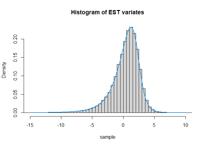
sample = rmvEST(n = 1e5,mu = 2,Sigma = 5,lambda = -2,tau = 0.5,nu = 4)
print(head(sample))
#> [1] -0.5015923 -0.6642021 0.2891897 3.5957041 2.9828134 3.4525520
#plotting
hist(sample,breaks = 150,freq = FALSE,xlim = c(-15,10),main = "Histogram of EST variates")
curve(expr = dmvEST(x,mu = 2,Sigma = 5,lambda = -2,tau = 0.5,nu = 4),
from = -15,to = 10,n = 200,lwd = 2,col = 4,add = TRUE)
#Multivariate case
mu = c(0.1,0.2,0.3,0.4)
Sigma = matrix(data = c(1,0.2,0.3,0.1,0.2,1,0.4,-0.1,0.3,0.4,1,0.2,0.1,-0.1,0.2,1),
               nrow = length(mu),ncol = length(mu),byrow = TRUE)
lambda = c(-2,0,1,2)

#One observation
dmvSN(x = c(-2,-1,0,1),mu,Sigma,lambda) #Skew-normal
#> [1] 0.003279037
rmvST(n = 10,mu,Sigma,lambda,nu = 2) #Skew-t
#>              [,1]        [,2]      [,3]       [,4]
#>  [1,]  0.35393287  0.18670145 0.7951902  0.3964539
#>  [2,] -1.22145843  1.98821902 2.2555133  2.4771210
#>  [3,]  0.11505972  0.18907948 0.2638879  0.4822362
#>  [4,] -0.79663450  1.12417008 1.2132558 -0.3534125
#>  [5,] -0.27912920  0.17194797 0.1671234  0.3730229
#>  [6,]  0.27243028 -0.01265475 0.9086517  0.3656542
#>  [7,]  0.41908397  0.77848822 0.3260464  0.7753323
#>  [8,]  0.78939078  0.74624772 1.3954601  0.5453789
#>  [9,]  0.03073276  0.65275698 1.2502771  0.3931312
#> [10,]  0.47251536  0.17043266 1.7512018  0.7576431

#Many observations as matrix
x = matrix(rnorm(4*10),ncol = 4,byrow = TRUE)
dmvST(x = x,mu,Sigma,lambda,nu = 2) #Skew-t
#>  [1] 7.255175e-07 2.994456e-04 3.493918e-03 3.356577e-06 2.428353e-03
#>  [6] 3.762044e-05 2.284900e-02 1.217553e-02 3.003915e-02 1.311547e-06

# Probability between some points
lower = rep(-5,4)
upper = c(-1,0,2,5)
pmvSN(lower,upper,mu,Sigma,lambda) #Skew-normal
#> [1] 0.123428
pmvST(lower,upper,mu,Sigma,lambda,nu=2) #Skew-t
#> [1] 0.1335012
The pmvSN() and pmvESN() functions offer
the option to return the logarithm in base 2 of the probability, useful
when the true probability is too small for the machine precision. These
functions above use methods in Genz (1992) through the
mvtnorm package (linked directly to our C++
functions) and Cao et al. (2019) through the package
tlrmvnmvt.
For this purpose, we call the function meanvarTMD()
which returns the mean vector and variance-covariance matrix for some
doubly truncated skew-elliptical distributions. It supports the -variate
Normal, Skew-normal (SN), Extended Skew-normal (ESN) and Unified
Skew-normal (SUN) as well as the Student’s-t, Skew-t (ST), Extended
Skew-t (EST) and Unified Skew-t (SUT) distribution. The distribution to
be used is set by the argument dist. Next, we present some
sample codes.
a = c(-0.8,-0.7,-0.6)
b = c(0.5,0.6,0.7)
mu = c(0.1,0.2,0.3)
Sigma = matrix(data = c(1,0.2,0.3,0.2,1,0.4,0.3,0.4,1),
               nrow = length(mu),ncol = length(mu),byrow = TRUE)

# Theoretical value
value1 = meanvarTMD(a,b,mu,Sigma,dist="normal")

#MC estimate
MC11 = MCmeanvarTMD(a,b,mu,Sigma,dist="normal") #by defalut n = 10000
MC12 = MCmeanvarTMD(a,b,mu,Sigma,dist="normal",n = 10^5) #more precision

# Now works for for any nu>0
value2 = meanvarTMD(a,b,mu,Sigma,dist = "t",nu = 0.87)

value3 = meanvarTMD(a,b,mu,Sigma,lambda = c(-2,0,1),dist = "SN")
value4 = meanvarTMD(a,b,mu,Sigma,lambda = c(-2,0,1),nu = 4,dist = "ST")
value5 = meanvarTMD(a,b,mu,Sigma,lambda = c(-2,0,1),tau = 1,dist = "ESN")
value6 = meanvarTMD(a,b,mu,Sigma,lambda = c(-2,0,1),tau = 1,nu = 4,dist = "EST")

#Skew-unified Normal (SUN) and Skew-unified t (SUT) distributions

Lambda = matrix(c(1,0,2,-3,0,-1),3,2) #A skewness matrix p times q
Gamma  = matrix(c(1,-0.5,-0.5,1),2,2) #A correlation matrix q times q
tau    = c(-1,2)                      #A vector of extension parameters of dim q

value7 = meanvarTMD(a,b,mu,Sigma,lambda = Lambda,tau = c(-1,2),Gamma = Gamma,dist = "SUN")
value8 = meanvarTMD(a,b,mu,Sigma,lambda = Lambda,tau = c(-1,2),Gamma = Gamma,nu = 4,dist = "SUT")


#The ESN and EST as particular cases of the SUN and SUT for q=1

Lambda = matrix(c(-2,0,1),3,1)
Gamma  = 1
value9 = meanvarTMD(a,b,mu,Sigma,lambda = Lambda,tau = 1,Gamma = Gamma,dist = "SUN")
value10 = meanvarTMD(a,b,mu,Sigma,lambda = Lambda,tau = 1,Gamma = Gamma,nu = 4,dist = "SUT")

round(value5$varcov,2) == round(value9$varcov,2)
#>      [,1] [,2] [,3]
#> [1,] TRUE TRUE TRUE
#> [2,] TRUE TRUE TRUE
#> [3,] TRUE TRUE TRUE
round(value6$varcov,2) == round(value10$varcov,2)
#>      [,1] [,2] [,3]
#> [1,] TRUE TRUE TRUE
#> [2,] TRUE TRUE TRUE
#> [3,] TRUE TRUE TRUE
As noted in the codes above, it is possible to obtain the moments by
Monte Carlo approximation through the MCmeanvarTMD()
function.
Finally, the momentsTMD provides the product moment for
some truncated multivariate distributions. For instance, in order to
compute the moment
𝔼[Y13Y21Y32 | a1≤Y1≤b1, a2≤Y2≤b2, a3≤Y3≤b3],
for
Y = (Y1,Y2,Y3)⊤ ∼ ESN3(μ,Σ,λ,τ),
we run the following code:
momentsTMD(kappa = c(3,1,2),lower = a,upper = b,mu,Sigma,lambda = c(-2,0,1),tau = 1,dist = "ESN")
#>    k1 k2 k3          E[k]
#> 1   0  0  0  1.0000000000
#> 2   1  0  0 -0.1955214032
#> 3   2  0  0  0.1604269300
#> 4   3  0  0 -0.0737276819
#> 5   0  1  0 -0.0284407326
#> 6   1  1  0  0.0075618650
#> 7   2  1  0 -0.0052312893
#> 8   3  1  0  0.0027692663
#> 9   0  0  1  0.1125134640
#> 10  1  0  1 -0.0041546757
#> 11  2  0  1  0.0130889137
#> 12  3  0  1 -0.0030069873
#> 13  0  1  1  0.0048928388
#> 14  1  1  1 -0.0012302466
#> 15  2  1  1  0.0008848539
#> 16  3  1  1 -0.0004097346
#> 17  0  0  2  0.1390876665
#> 18  1  0  2 -0.0249750438
#> 19  2  0  2  0.0219172190
#> 20  3  0  2 -0.0096157104
#> 21  0  1  2 -0.0026900254
#> 22  1  1  2  0.0008924818
#> 23  2  1  2 -0.0005106163
#> 24  3  1  2  0.0003672320
Note that some other lower order moments involved in the computation are also returned.
Functions for the folded cases are also offered to the users. The
analogous functions meanvarFMD(), momentsFMD()
are used for the mean and variance-covariance matrix, and arbitrary
product moments, respectively. Besides, the cdfFMD()
computes the cdf. The available distributions are normal, Student-t, SN
and ESN being set by the argument dist. Some sample codes
are shown next.
mu = c(0.1,0.2,0.3,0.4)
Sigma = matrix(data = c(1,0.2,0.3,0.1,0.2,1,0.4,-0.1,0.3,0.4,1,0.2,0.1,-0.1,0.2,1),
               nrow = length(mu),ncol = length(mu),byrow = TRUE)

#cdf
cdfFMD(x = c(0.5,0.2,1.0,1.3),mu,Sigma,lambda = c(-2,0,2,1),dist = "SN")
#> [1] 0.02794654

#Mean and variance-covariance matrix
meanvarFMD(mu,Sigma,dist = "t",nu = 4)
#> $mean
#>          [,1]
#> [1,] 1.003746
#> [2,] 1.014938
#> [3,] 1.033438
#> [4,] 1.059027
#>
#> $EYY
#>          [,1]     [,2]     [,3]     [,4]
#> [1,] 2.010000 1.316949 1.367027 1.335528
#> [2,] 1.316949 2.040000 1.430244 1.338320
#> [3,] 1.367027 1.430244 2.090000 1.392964
#> [4,] 1.335528 1.338320 1.392964 2.160000
#>
#> $varcov
#>           [,1]      [,2]      [,3]      [,4]
#> [1,] 1.0024938 0.2982090 0.3297167 0.2725335
#> [2,] 0.2982090 1.0099010 0.3813678 0.2634737
#> [3,] 0.3297167 0.3813678 1.0220049 0.2985250
#> [4,] 0.2725335 0.2634737 0.2985250 1.0384615

#Product moment c(2,0,1,2)
momentsFMD(kappa = c(2,0,1,2),mu,Sigma,lambda = c(-2,0,2,1),tau = 1,dist = "ESN")
#>    k1 k2 k3 k4      E[k]
#> 1   2  0  1  2 1.3147576
#> 2   1  0  1  2 1.0309879
#> 3   0  0  1  2 1.2496227
#> 4   2  0  0  2 1.1854733
#> 5   1  0  0  2 0.9932095
#> 6   0  0  0  2 1.3074975
#> 7   2  0  1  1 0.8707904
#> 8   1  0  1  1 0.6921804
#> 9   0  0  1  1 0.8518643
#> 10  2  0  0  1 0.8261674
#> 11  1  0  0  1 0.6949156
#> 12  0  0  0  1 0.9196535
#> 13  2  0  1  0 0.8847480
#> 14  1  0  1  0 0.7128806
#> 15  0  0  1  0 0.8925955
#> 16  2  0  0  0 0.8956343
#> 17  1  0  0  0 0.7535822
#> 18 0 0 0 0 1.0000000Cao, J., Genton, M. G., Keyes, D. E., & Turkiyyah, G. M. “Exploiting Low Rank Covariance Structures for Computing High-Dimensional Normal and Student- t Probabilities” (2019) https://marcgenton.github.io/2019.CGKT.manuscript.pdf
Galarza, C. E., Lin, T. I., Wang, W. L., & Lachos, V. H. (2021). On moments of folded and truncated multivariate Student-t distributions based on recurrence relations. Metrika, 84(6), 825-850.
Galarza-Morales, C. E., Matos, L. A., Dey, D. K., & Lachos, V. H. (2022a). “On moments of folded and doubly truncated multivariate extended skew-normal distributions.” Journal of Computational and Graphical Statistics, 1-11 doi:10.1080/10618600.2021.2000869.
Galarza, C. E., Matos, L. A., Castro, L. M., & Lachos, V. H. (2022b). Moments of the doubly truncated selection elliptical distributions with emphasis on the unified multivariate skew-t distribution. Journal of Multivariate Analysis, 189, 104944 doi:10.1016/j.jmva.2021.104944.
Genz, A. (1992), “Numerical computation of multivariate normal probabilities,” Journal of Computational and Graphical Statistics, 1, 141-149.
Kan, R., & Robotti, C. (2017). On moments of folded and truncated multivariate normal distributions. Journal of Computational and Graphical Statistics, 26(4), 930-934.