![]()
The jti package (pronounced ‘yeti’) is a memory
efficient implementaion of the junction tree algorithm (JTA) using the
Lauritzen-Spiegelhalter scheme. Why is it memory efficient? Because we
use a for the potentials which enable us to
handle large and complex graphs where the variables can have an
arbitrary large number of levels. The jti package is a
big part of the software paper
.
Current stable release from CRAN:
install.packages("jti")Development version (see README.md for new
features):
devtools::install_github("mlindsk/jti", build_vignettes = FALSE)library(jti)
library(igraph)el <- matrix(c(
"A", "T",
"T", "E",
"S", "L",
"S", "B",
"L", "E",
"E", "X",
"E", "D",
"B", "D"),
nc = 2,
byrow = TRUE
)
g <- igraph::graph_from_edgelist(el)
plot(g)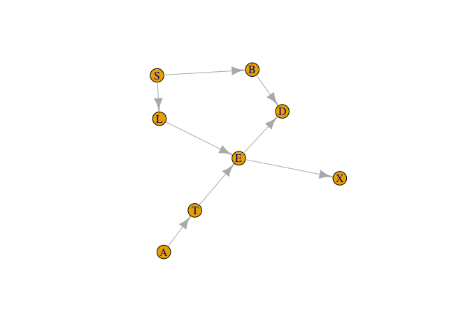
We use the asia data; see the man page (?asia)
Checking and conversion
cl <- cpt_list(asia, g)
cl
#>  List of CPTs
#>  -------------------------
#>   P( A )
#>   P( T | A )
#>   P( E | T, L )
#>   P( S )
#>   P( L | S )
#>   P( B | S )
#>   P( X | E )
#>   P( D | E, B )
#>
#>   <bn_, cpt_list, list>
#>  -------------------------
Compilation
cp <- compile(cl)
cp
#>  Compiled network  (cpts initialized)
#>  ------------------------------------
#>   Nodes: 8
#>   Cliques: 6
#>    - max: 3
#>    - min: 2
#>    - avg: 2.67
#>   <bn_, charge, list>
#>  ------------------------------------
# plot(get_graph(cp)) # Should give the same as plot(g)
After the network has been compiled, the graph has been triangulated and moralized. Furthermore, all conditional probability tables (CPTs) has been designated to one of the cliques (in the triangulated and moralized graph).
jt1 <- jt(cp)
jt1
#> Junction Tree
#> -------------------------
#> Propagated: full
#> Flow: sum
#> Cliques: 6
#> - max: 3
#> - min: 2
#> - avg: 2.67
#> <jt, list>
#> -------------------------
plot(jt1)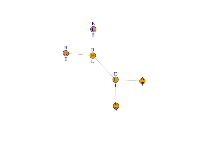 Query probabilities
query_belief(jt1, c("E", "L", "T"))
#> $E
#> E
#>         n         y
#> 0.9257808 0.0742192
#>
#> $L
#> L
#>     n     y
#> 0.934 0.066
#>
#> $T
#> T
#>      n      y
#> 0.9912 0.0088
query_belief(jt1, c("B", "D", "E"), type = "joint")
#> , , B = y
#>
#>    E
#> D            n           y
#>   y 0.36261346 0.041523361
#>   n 0.09856873 0.007094444
#>
#> , , B = n
#>
#>    E
#> D            n           y
#>   y 0.04637955 0.018500278
#>   n 0.41821906 0.007101117
It should be noticed, that the above could also have been achieved by
jt1 <- jt(cp, propagate = "no")
jt1 <- propagate(jt1, prop = "full")
That is; it is possible to postpone the actual propagation.
e2  <- c(A = "y", X = "n")
jt2 <- jt(cp, e2)
query_belief(jt2, c("B", "D", "E"), type = "joint")
#> , , B = y
#>
#>    E
#> D           n            y
#>   y 0.3914092 3.615182e-04
#>   n 0.1063963 6.176693e-05
#>
#> , , B = n
#>
#>    E
#> D            n            y
#>   y 0.05006263 2.009085e-04
#>   n 0.45143057 7.711638e-05
Notice that, the configuration (D,E,B) = (y,y,n) has
changed dramatically as a consequence of the evidence. We can get the
probability of the evidence:
query_evidence(jt2)
#> [1] 0.007152638jt3 <- jt(cp, flow = "max")
mpe(jt3)
#> A T E L S B X D
#> "n" "n" "n" "n" "n" "n" "n" "n"e4 <- c(T = "y", X = "y", D = "y")
jt4 <- jt(cp, e4, flow = "max")
mpe(jt4)
#> A T E L S B X D
#> "n" "y" "y" "n" "y" "y" "y" "y"Notice, that T, E, S,
B, X and D has changed from
"n" to "y" as a consequence of the new
evidence e4.
cp5 <- compile(cpt_list(asia, g) , root_node = "X")
jt5 <- jt(cp5, propagate = "collect")
We can only query from the variables in the root clique now but we
have ensured that the node of interest, “X”, does indeed live in this
clique. The variables are found using get_clique_root.
query_belief(jt5, get_clique_root(jt5), "joint")
#>    E
#> X            n            y
#>   n 0.88559032 0.0004011849
#> y 0.04019048 0.0738180151cl <- cpt_list(asia2)
cp6 <- compile(cl)Inspection; see if the graph correspond to the cpts
plot(get_graph(cp6)) 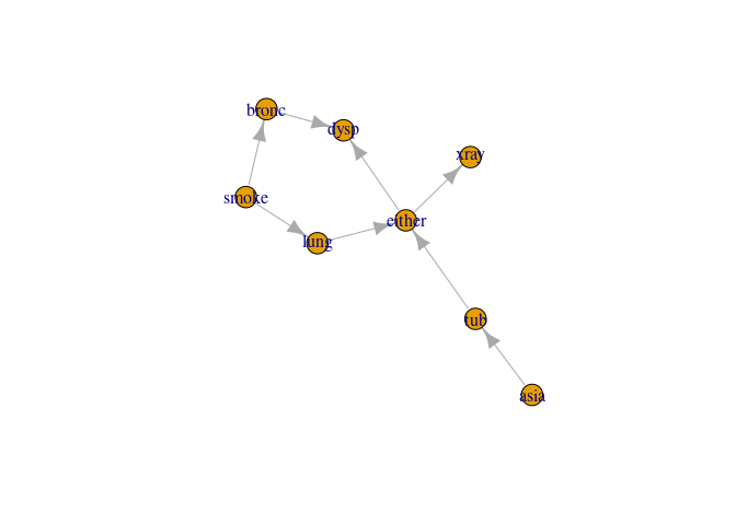
This time we specify that no propagation should be performed
jt6 <- jt(cp6, propagate = "no")We can now inspect the collecting junction tree and see which cliques are leaves and parents
plot(jt6)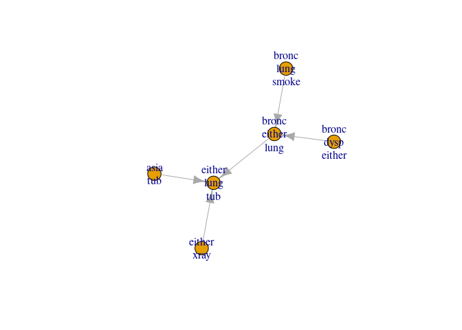
get_cliques(jt6)
#> $C1
#> [1] "asia" "tub"
#>
#> $C2
#> [1] "either" "lung"   "tub"
#>
#> $C3
#> [1] "bronc"  "either" "lung"
#>
#> $C4
#> [1] "bronc" "lung"  "smoke"
#>
#> $C5
#> [1] "bronc"  "dysp"   "either"
#>
#> $C6
#> [1] "either" "xray"
get_clique_root(jt6)
#> [1] "either" "lung"   "tub"
jt_leaves(jt6)
#> [1] 1 4 5 6
unlist(jt_parents(jt6))
#> [1] 2 3 3 2
That is; - clique 2 is parent of clique 1 - clique 3 is parent of clique 4 etc.
Next, we send the messages from the leaves to the parents
jt6 <- send_messages(jt6)Inspect again
plot(jt6)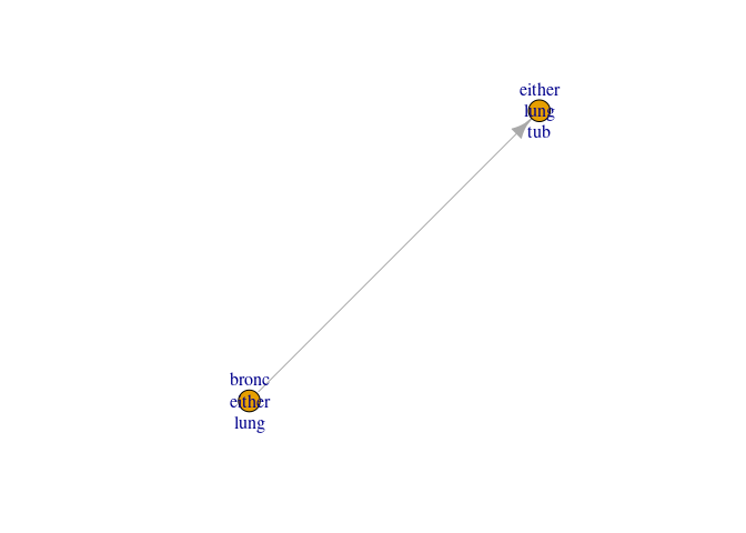
Send the last message to the root and inspect
jt6 <- send_messages(jt6)
plot(jt6)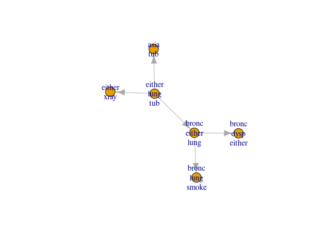
The arrows are now reversed and the outwards (distribute) phase begins
jt_leaves(jt6)
#> [1] 2
jt_parents(jt6)
#> [[1]]
#> [1] 1 3 6
Clique 2 (the root) is now a leave and it has 1, 3 and 6 as parents. Finishing the message passing
jt6 <- send_messages(jt6)
jt6 <- send_messages(jt6)
Queries can now be performed as normal
query_belief(jt6, c("either", "tub"), "joint")
#>       tub
#> either    yes       no
#>    yes 0.0104 0.054428
#> no 0.0000 0.935172We use the ess package (on CRAN), found at https://github.com/mlindsk/ess, to fit an undirected
decomposable graph to data.
library(ess)

g7  <- ess::fit_graph(asia, trace = FALSE)
ig7 <- ess::as_igraph(g7)
cp7 <- compile(pot_list(asia, ig7))
jt7 <- jt(cp7)

query_belief(jt7, get_cliques(jt7)[[4]], type = "joint")
#> , , T = n
#>
#>    L
#> E       n      y
#>   n 0.926 0.0000
#>   y 0.000 0.0652
#>
#> , , T = y
#>
#>    L
#> E       n     y
#>   n 0.000 0e+00
#>   y 0.008 8e-04