![]()
![]()
An R package for univariate kernel density estimation
with parametric starts and asymmetric kernels.
kdensity is now linked to univariateML,
meaning it supports the approximately 30+ parametric starts from that
package!
kdensity is an implementation of univariate kernel density estimation
with support for parametric starts and asymmetric kernels. Its main
function is kdensity, which is has approximately the same
syntax as stats::density. Its new functionality is:
kdensity has built-in support for many parametric
starts, such as normal and gamma, but you
can also supply your own. For a list of supported parametric starts, see
the readme of univariateML.gcopula and gamma kernels, but also the common
symmetric ones. In addition, you can also supply your own kernels.bw,
again including an option to specify your own.A reason to use kdensity is to avoid boundary
bias when estimating densities on the unit interval or the positive
half-line. Asymmetric kernels such as gamma and
gcopula are designed for this purpose. The support for
parametric starts allows you to easily use a method that is often
superior to ordinary kernel density estimation.
Several R packages deal with kernel estimation. For an
overview see Deng &
Hadley Wickham (2011). While no other R package handles
density estimation with parametric starts, several packages supports
methods that handle boundary bias. evmix
provides a variety of boundary bias correction methods in the
bckden function. kde1d corrects
for boundary bias using transformed univariate local polynomial kernel
density estimation. logKDE
corrects for boundary bias on the half line using a logarithmic
transform. ks
supports boundary correction through the kde.boundary
function, while Ake
corrects for boundary bias using tailored kernel functions.
From inside R, use one of the following commands:
# For the CRAN release
install.packages("kdensity")
# For the development version from GitHub:
# install.packages("devtools")
devtools::install_github("JonasMoss/kdensity")Call the library function and use it just like
stats::density, but with optional additional arguments.
library("kdensity")
plot(kdensity(mtcars$mpg, start = "normal"))Kernel density estimation with a parametric start was introduced by Hjort and Glad in Nonparametric Density Estimation with a Parametric Start (1995). The idea is to start out with a parametric density before you do your kernel density estimation, so that your actual kernel density estimation will be a correction to the original parametric estimate. The resulting estimator will outperform the ordinary kernel density estimator in terms of asymptotic integrated mean squared error whenever the true density is close to your suggestion; and the estimator can be superior to the ordinary kernel density estimator even when the suggestion is pretty far off.
In addition to parametric starts, the package implements some asymmetric kernels. These kernels are useful when modelling data with sharp boundaries, such as data supported on the positive half-line or the unit interval. Currently we support the following asymmetric kernels:
Jones and Henderson’s Gaussian copula KDE, from
Kernel-Type Density Estimation on the Unit Interval (2007)). This is
used for data on the unit interval. The bandwidth selection mechanism
described in that paper is implemented as well. This kernel is called
gcopula.
Chen’s two beta kernels from Beta kernel estimators for
density functions (1999). These are used for data supported on the on
the unit interval, and are called beta and
beta_biased.
Chen’s two gamma kernels from Probability Density
Function Estimation Using Gamma Kernels (2000). These are used for data
supported on the positive half-line, and are called gamma
and gamma_biased.
These features can be combined to make asymmetric kernel densities
estimators with parametric starts, see the example below. The package
contains only one function, kdensity, in addition to the
generics plot, points, lines,
summary, and print.
The function kdensity takes some data, a
kernel kernel and a parametric start start.
You can optionally specify the support parameter, which is
used to find the normalizing constant.
The following example uses the data set. The black curve is a
gamma-kernel density estimate with a gamma start, the red curve a fully
parametric gamma density and and the blue curve an ordinary
density estimate. Notice the boundary bias of the ordinary
density estimator. The underlying parameter estimates are
always maximum likelilood.
library("kdensity")
kde = kdensity(airquality$Wind, start = "gamma", kernel = "gamma")
plot(kde, main = "Wind speed (mph)")
lines(kde, plot_start = TRUE, col = "red")
lines(density(airquality$Wind, adjust = 2), col = "blue")
rug(airquality$Wind)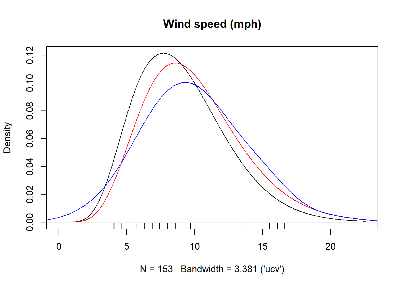
Since the return value of kdensity is a function,
kde is callable and can be used as any density function in
R (such as stats::dnorm). For example, you can
do:
kde(10)
#> [1] 0.09980471
integrate(kde, lower = 0, upper = 1) # The cumulative distribution up to 1.
#> 1.27532e-05 with absolute error < 2.2e-19
You can access the parameter estimates by using coef.
You can also access the log likelihood (logLik), AIC and
BIC of the parametric start distribution.
coef(kde)
#> Maximum likelihood estimates for the Gamma model
#>  shape    rate
#> 7.1873  0.7218
logLik(kde)
#> 'log Lik.' 12.33787 (df=2)
AIC(kde)
#> [1] -20.67574If you encounter a bug, have a feature request or need some help, open a Github issue. Create a pull requests to contribute. This project follows a Contributor Code of Conduct.
[Jones, M. C., and D. A. Henderson. “Miscellanea kernel-type density estimation on the unit interval.” Biometrika 94.4 (2007):977-984.]
[Chen, Song Xi. “Beta kernel estimators for density functions.” Computational Statistics & Data Analysis 31.2 (1999):131-145.]