| Title: | Dynamic Multi-Species Size Spectrum Modelling |
| Date: | 2026-08-31 |
| Type: | Package |
| Description: | A set of classes and methods to set up and run multi-species, trait based and community size spectrum ecological models, focused on the marine environment. |
| Maintainer: | Gustav Delius <gustav.delius@york.ac.uk> |
| Version: | 3.4.0 |
| License: | GPL-3 |
| Imports: | assertthat, deSolve, dplyr, ggplot2 (≥ 3.4.0), ggrepel, grid, lubridate, methods, nleqslv, plotly, plyr, progress, Rcpp, reshape2, rlang, lifecycle, pak |
| LinkingTo: | Rcpp |
| Depends: | R (≥ 3.5) |
| Suggests: | testthat (≥ 3.0.0), withr, vdiffr, diffviewer, roxygen2, knitr, rmarkdown, quarto, pkgdown, covr, spelling |
| Collate: | 'age_mat.R' 'helpers.R' 'info_signals.R' 'MizerParams-class.R' 'MizerSim-class.R' 'registerExtensions.R' 'ArraySpeciesBySize-class.R' 'ArrayTimeBySpecies-class.R' 'ArrayTimeBySpeciesBySize-class.R' 'ArrayResourceBySize-class.R' 'MizerScan-class.R' 'generic_methods.R' 'background.R' 'reproduction.R' 'saveParams.R' 'species_params.R' 'getRequiredRDD.R' 'setColours.R' 'setInteraction.R' 'setPredKernel.R' 'setSearchVolume.R' 'setMaxIntakeRate.R' 'setMetabolicRate.R' 'setMetadata.R' 'setExtMort.R' 'setExtEncounter.R' 'diffusion.R' 'second_order_w.R' 'setExtDiffusion.R' 'setReproduction.R' 'setResource.R' 'setFishing.R' 'setInitialValues.R' 'setBevertonHolt.R' 'upgrade.R' 'selectivity_funcs.R' 'pred_kernel_funcs.R' 'resource_dynamics.R' 'resource_semichemostat.R' 'resource_logistic.R' 'numerical_methods.R' 'transport.R' 'project_n.R' 'project.R' 'mizer-package.R' 'project_methods.R' 'rate_functions.R' 'sim_rates.R' 'sizeIntegral.R' 'summary_methods.R' 'indicator_functions.R' 'plots.R' 'plotBiomassObservedVsModel.R' 'plotYieldObservedVsModel.R' 'animateSpectra.R' 'newMultispeciesParams.R' 'wrapper_functions.R' 'newSingleSpeciesParams.R' 'steady.R' 'steadyState.R' 'scanModel.R' 'scan_setters.R' 'plotYieldVsF.R' 'extension.R' 'data.R' 'RcppExports.R' 'deprecated.R' 'get_initial_n.R' 'compareParams.R' 'customFunction.R' 'manipulate_species.R' 'observations.R' 'calibrate.R' 'scaleRates.R' 'match.R' 'matchGrowth.R' 'steadySingleSpecies.R' 'steadyNewton.R' 'getSteadyResidual.R' 'getOscillationModeSim.R' 'defaults_edition.R' 'validSpeciesParams.R' 'zzz.R' |
| Encoding: | UTF-8 |
| LazyData: | true |
| URL: | https://sizespectrum.org/mizer/, https://github.com/sizespectrum/mizer |
| BugReports: | https://github.com/sizespectrum/mizer/issues |
| Language: | en-GB |
| RdMacros: | lifecycle |
| VignetteBuilder: | knitr, quarto |
| Config/testthat/edition: | 3 |
| Config/testthat/parallel: | true |
| Config/testthat/start-first: | steadyState, steadyNewton, getOscillationModeSim, rate_functions, steady, plots, manipulate_species |
| Config/roxygen2/version: | 8.1.0 |
| NeedsCompilation: | yes |
| Packaged: | 2026-08-31 02:38:00 UTC; gustav |
| Author: | Gustav Delius  [cre, aut, cph],
Finlay Scott [aut, cph],
Julia Blanchard
[aut, cph],
Ken Andersen
[aut, cph],
Richard Southwell [ctb, cph]
[cre, aut, cph],
Finlay Scott [aut, cph],
Julia Blanchard
[aut, cph],
Ken Andersen
[aut, cph],
Richard Southwell [ctb, cph] |
| Repository: | CRAN |
| Date/Publication: | 2026-08-31 16:00:03 UTC |
mizer: Multi-species size-based modelling in R
Description
The mizer package implements multi-species size-based modelling in R. It has been designed for modelling marine ecosystems.
Details
Using mizer is relatively simple. There are three main stages:
-
Setting the model parameters. This is done by creating an object of class MizerParams. This includes model parameters such as the life history parameters of each species, and the range of the size spectrum. There are several setup functions that help to create a MizerParams objects for particular types of models:
-
Running a simulation. This is done by calling the
project()function with the model parameters. This produces an object of MizerSim that contains the results of the simulation. -
Exploring results. After a simulation has been run, the results can be explored using a range of plotting_functions, summary_functions and indicator_functions.
See the mizer website for full details of the principles behind mizer and how the package can be used to perform size-based modelling.
Author(s)
Maintainer: Gustav Delius gustav.delius@york.ac.uk (ORCID) [copyright holder]
Authors:
Gustav Delius gustav.delius@york.ac.uk (ORCID) [copyright holder]
Finlay Scott drfinlayscott@gmail.com [copyright holder]
Julia Blanchard julia.blanchard@utas.edu.au (ORCID) [copyright holder]
Ken Andersen kha@aqua.dtu.dk (ORCID) [copyright holder]
Other contributors:
Richard Southwell richard.southwell@york.ac.uk [contributor, copyright holder]
See Also
Useful links:
Report bugs at https://github.com/sizespectrum/mizer/issues
Check that a rate function returns the correct output dimensions
Description
Called by setRateFunction() to verify that a candidate rate function
returns an array (or vector/list) of the correct dimensions for the
requested rate.
Usage
.checkRateFunctionOutput(params, rate, fun)
Arguments
params |
A MizerParams object |
rate |
Name of the rate being replaced, e.g. |
fun |
Name of the candidate function to validate. |
Value
Invisibly NULL. Called for its side-effect of stopping with an
informative error if the output has the wrong shape.
S4/S3 compatibility .hasSlot helper
Description
S4/S3 compatibility .hasSlot helper
Usage
.hasSlot(object, name)
Arguments
object |
An object (S4 or S3). |
name |
Name of the slot / list element. |
Value
Logical.
S3 class for resource size spectra
Description
![[Experimental]](./figures/lifecycle-experimental.svg) Several functions in mizer return a vector over the full size grid holding
a resource-related quantity such as the resource number density, the
resource mortality, the intrinsic resource birth rate or carrying capacity.
The
Several functions in mizer return a vector over the full size grid holding
a resource-related quantity such as the resource number density, the
resource mortality, the intrinsic resource birth rate or carrying capacity.
The ArrayResourceBySize class wraps these vectors to provide convenient
print(), summary(), plot(), and as.data.frame() methods.
Usage
ArrayResourceBySize(
  x,
  value_name = NULL,
  units = NULL,
  type = NULL,
  params = NULL
)

is.ArrayResourceBySize(x)
Arguments
x |
A numeric vector over the full size grid. For
|
value_name |
A string giving the human-readable name for the value. |
units |
A string giving the units (e.g. "1/year"). |
type |
The kind of quantity the values are, see |
params |
A |
Details
An ArrayResourceBySize object behaves just like a regular numeric vector
for arithmetic operations and subsetting. It carries three lightweight
attributes:
-
value_name– a human-readable name for the value (e.g. "Resource mortality"). -
units– the units of the value (e.g. "1/year"). -
params– theMizerParamsobject that the value was computed from.
Value
An ArrayResourceBySize object (inherits from numeric).
is.ArrayResourceBySize() returns TRUE if x is an
ArrayResourceBySize object, FALSE otherwise.
See Also
print(), summary(), as.data.frame(), plot(), plot2(),
plotRelative(), addPlot()
Examples
mort <- getResourceMort(NS_params)
is.ArrayResourceBySize(mort)
summary(mort)
plot(mort)
The complete plotting data of a resource-by-size array
Description
The resource analogue of ArraySpeciesBySize_plot_data(): the weight limits,
the conversion of the values and of the size coordinate onto the requested
axis, and the length limits, all done with the array's own params. A
resource array holds a single spectrum, so there is no selection, no
background and no total to form.
Usage
ArrayResourceBySize_plot_data(
  x,
  wlim = c(NA, NA),
  llim = c(NA, NA),
  size_axis = "w",
  per_log_size = NULL
)
Arguments
x |
An |
wlim |
Numeric vector of length two giving the weight limits. |
llim |
Numeric vector of length two giving the length limits, applied only on a length axis. |
size_axis |
Either |
per_log_size |
Whether to express a density per logarithmic size. |
Value
A data frame with the size coordinate in its first column, the values
in its second, and Species and Legend columns.
S3 class for species x size rate arrays
Description
Many functions in mizer return two-dimensional arrays (species x size)
holding rates like encounter rate, feeding level, growth rate, mortality etc.
The ArraySpeciesBySize class wraps these arrays to provide convenient
print(), summary(), plot(), and as.data.frame() methods.
Usage
ArraySpeciesBySize(
  x,
  value_name = NULL,
  units = NULL,
  type = NULL,
  params = NULL,
  representation = c("point", "average")
)

is.ArraySpeciesBySize(x)
Arguments
x |
A matrix (species x size). For |
value_name |
A string giving the human-readable name for the value. |
units |
A string giving the units (e.g. "g/year", "1/year"). |
type |
The kind of quantity the values are, see array_types:
|
params |
A |
representation |
Either |
Details
An ArraySpeciesBySize object behaves just like a regular matrix for
arithmetic operations and subsetting. It carries a few lightweight
attributes:
-
value_name– a human-readable name for the value (e.g. "Encounter rate"). -
units– the units of the rate (e.g. "g/year"). -
type– the kind of quantity the values are.
Value
An ArraySpeciesBySize object (inherits from matrix and array).
is.ArraySpeciesBySize() returns TRUE if x is an
ArraySpeciesBySize object, FALSE otherwise.
See Also
print(), summary(), as.data.frame(), plot()
Examples
enc <- getEncounter(NS_params)
is.ArraySpeciesBySize(enc)
summary(enc)
The complete plotting data of a species-by-size array
Description
Everything a plot of an ArraySpeciesBySize needs, prepared once: the
species selection, the background grouping, the masking of sizes outside a
species' own range, the weight limits, the conversion of the values and of
the size coordinate onto the requested axis, the total line, and the length
limits.
Usage
ArraySpeciesBySize_plot_data(
  x,
  species = NULL,
  all.sizes = FALSE,
  wlim = c(NA, NA),
  llim = c(NA, NA),
  total = FALSE,
  background = TRUE,
  size_axis = "w",
  per_log_size = NULL
)
Arguments
x |
An |
species |
Character vector of species to include, or |
all.sizes |
If |
wlim |
Numeric vector of length two giving the weight limits. |
llim |
Numeric vector of length two giving the length limits, applied only on a length axis. |
total |
Whether to append the total line, see |
background |
Whether background species are included. |
size_axis |
Either |
per_log_size |
Whether to express a density per logarithmic size. |
Details
All of it uses the array's own params. That matters for the comparison
plots, where the two operands may come from different models: a length axis
and a density Jacobian are both built from the weight-length relationship of
the model the values came from, so preparing the second array with the first
one's parameters would put it in the wrong place on the axis. Each operand is
therefore prepared here, on its own, and the comparison renderers receive
data that is already on the axis it will be drawn against.
Value
A data frame with the size coordinate in its first column, the values
in its second, and Species and Legend columns.
S3 class for time x resource-size arrays
Description
The NResource() function returns a two-dimensional array (time x size)
holding the resource number density through time. The
ArrayTimeByResourceBySize class wraps this array to provide convenient
print(), summary(), plot(), and as.data.frame() methods.
Usage
ArrayTimeByResourceBySize(
  x,
  value_name = NULL,
  units = NULL,
  type = NULL,
  params = NULL
)

is.ArrayTimeByResourceBySize(x)
Arguments
x |
A matrix (time x size). For |
value_name |
A string giving the human-readable name for the value. |
units |
A string giving the units (e.g. "1/g"). |
type |
The kind of quantity the values are, see |
params |
A |
Details
An ArrayTimeByResourceBySize object behaves just like a regular matrix for
arithmetic operations and subsetting. It carries these lightweight
attributes:
-
value_name– a human-readable name for the value (e.g. "Number density"). -
units– the units of the value (e.g. "1/g"). -
params– theMizerParamsobject that the value was computed from.
Value
An ArrayTimeByResourceBySize object (inherits from matrix and
array).
is.ArrayTimeByResourceBySize() returns TRUE if x is an
ArrayTimeByResourceBySize object, FALSE otherwise.
See Also
print(), summary(), as.data.frame(), plot(), plot2(),
plotRelative(), addPlot(), animate()
Examples
nr <- NResource(NS_sim)
is.ArrayTimeByResourceBySize(nr)
summary(nr)
plot(nr)
S3 class for time x species arrays
Description
Some functions in mizer return two-dimensional arrays (time x species)
holding quantities like biomass, abundance, or yield rate through time.
The ArrayTimeBySpecies class wraps these arrays to provide convenient
print(), summary(), plot(), and as.data.frame() methods.
Usage
ArrayTimeBySpecies(
  x,
  value_name = NULL,
  units = NULL,
  type = NULL,
  params = NULL
)

is.ArrayTimeBySpecies(x)
Arguments
x |
A matrix (time x species). For |
value_name |
A string giving the human-readable name for the value. |
units |
A string giving the units (e.g. "g", "g/year"). |
type |
The kind of quantity the values are, see |
params |
A |
Details
An ArrayTimeBySpecies object behaves just like a regular matrix for
arithmetic operations and subsetting. It carries these lightweight attributes:
-
value_name– a human-readable name for the value (e.g. "Biomass"). -
units– the units of the value (e.g. "g", "g/year"). -
params– theMizerParamsobject that created the values.
Value
An ArrayTimeBySpecies object (inherits from matrix and array).
is.ArrayTimeBySpecies() returns TRUE if x is an
ArrayTimeBySpecies object, FALSE otherwise.
See Also
print(), summary(), as.data.frame(), plot()
Examples
bio <- getBiomass(NS_sim)
is.ArrayTimeBySpecies(bio)
summary(bio)
S3 class for time x species x size arrays
Description
Some functions in mizer return three-dimensional arrays (time x species x
size) holding quantities like fishing mortality, feeding level, or predation
mortality through time. The ArrayTimeBySpeciesBySize class wraps these
arrays to provide convenient print(), summary(), plot(),
animate(), and as.data.frame() methods.
Usage
ArrayTimeBySpeciesBySize(
  x,
  value_name = NULL,
  units = NULL,
  type = NULL,
  params = NULL,
  representation = c("point", "average")
)

is.ArrayTimeBySpeciesBySize(x)
Arguments
x |
A 3D array (time x species x size). For
|
value_name |
A string giving the human-readable name for the value. |
units |
A string giving the units (e.g. "1/year"). |
type |
The kind of quantity the values are, see |
params |
A |
representation |
Either |
Details
An ArrayTimeBySpeciesBySize object behaves just like a regular array for
arithmetic operations and subsetting. It carries these lightweight attributes:
-
value_name– a human-readable name for the value (e.g. "Fishing mortality"). -
units– the units of the value (e.g. "1/year"). -
type– the kind of quantity the values are. -
params– theMizerParamsobject that the value was computed from.
Value
An ArrayTimeBySpeciesBySize object (inherits from array).
is.ArrayTimeBySpeciesBySize() returns TRUE if x is an
ArrayTimeBySpeciesBySize object, FALSE otherwise.
See Also
print(), summary(), as.data.frame(), plot(),
animateSpectra()
Examples
fmort <- getFMort(NS_sim)
is.ArrayTimeBySpeciesBySize(fmort)
summary(fmort)
plot(fmort, time = 2007)
Beverton Holt function to calculate density-dependent reproduction rate
Description
Takes the density-independent rates R_{di} of egg production (as
calculated by getRDI()) and returns
reduced, density-dependent reproduction rates R_{dd} given as
R_{dd} = R_{di}
\frac{R_{max}}{R_{di} + R_{max}}
where
R_{max} are the maximum possible reproduction rates that must be
specified in a column in the species parameter dataframe.
(All quantities in the above equation are species-specific but we dropped
the species index for simplicity.)
Usage
BevertonHoltRDD(rdi, species_params, ...)
Arguments
rdi |
Vector of density-independent reproduction rates
|
species_params |
A species parameter dataframe. Must contain a column
|
... |
Unused |
Details
This is only one example of a density-dependence. You can write your own
function based on this example, returning different density-dependent
reproduction rates. Three other examples provided are RickerRDD(),
SheperdRDD(), noRDD() and constantRDD(). For more explanation see
setReproduction().
Value
Vector of density-dependent reproduction rates.
See Also
Other functions calculating density-dependent reproduction rate:
RickerRDD(),
SheperdRDD(),
constantEggRDI(),
constantRDD(),
noRDD()
Alias for set_multispecies_model()
Description
![[Deprecated]](./figures/lifecycle-deprecated.svg) An alias provided for backward compatibility with mizer version <= 1.0
An alias provided for backward compatibility with mizer version <= 1.0
Usage
MizerParams(
  species_params,
  interaction = matrix(1, nrow = nrow(species_params), ncol = nrow(species_params)),
  min_w_pp = 1e-10,
  min_w = 0.001,
  max_w = NULL,
  no_w = 100,
  n = 2/3,
  q = 0.8,
  f0 = 0.6,
  kappa = 1e+11,
  lambda = 2 + q - n,
  r_pp = 10,
  ...
)
Arguments
species_params |
A data frame of species-specific parameter values. |
interaction |
Optional interaction matrix of the species (predator species x prey species). By default all entries are 1. See "Setting interaction matrix" section below. |
min_w_pp |
The smallest size of the resource spectrum. By default this is set to the smallest value at which any of the consumers can feed. |
min_w |
Sets the size of the eggs of all species for which this is not
given in the |
max_w |
The largest size of the consumer spectrum. By default this is
set to the largest |
no_w |
The number of size bins in the consumer spectrum. |
n |
The allometric growth exponent. This can be overruled for individual
species by including a |
q |
Allometric exponent of search volume |
f0 |
Expected average feeding level. Used to set |
kappa |
The coefficient |
lambda |
Used to set power-law exponent for resource capacity if the
|
r_pp |
|
... |
Further arguments passed to |
Details
If species_params contains a w_inf column then it is copied to w_max.
If max_w is not supplied then it is set to 1.1 * max(species_params$w_max).
The supplied min_w_pp is shifted up by one grid step before being passed
to newMultispeciesParams() to compensate for the fact that newer mizer
versions extend the full size grid below min_w_pp.
Missing legacy columns in species_params are filled as follows:
gear = species, k = 0, alpha = 0.6, erepro = 1,
sel_func = "knife_edge", knife_edge_size = w_mat if needed,
catchability = 1, ks = h * 0.2, and m = 1.
If h is missing it is calculated from k_vb, alpha, f0 and w_max.
If gamma is missing it is calculated from f0, h, beta, sigma,
lambda and kappa.
Value
A MizerParams object
A class to hold the parameters for a size based model.
Description
Although it is possible to build a MizerParams object by hand it is
not recommended and several constructors are available. Dynamic simulations
are performed using project() function on objects of this class. As a
user you should never need to access the slots inside a MizerParams object
directly.
Details
The MizerParams class is fairly complex with a large number of
slots, many of which are multidimensional arrays. The dimensions of these
arrays is strictly enforced so that MizerParams objects are consistent
in terms of number of species and number of size classes.
The MizerParams class does not hold any dynamic information, e.g.
abundances or harvest effort through time. These are held in
MizerSim objects.
Slots
metadataA list with metadata information. See
setMetadata().mizer_versionThe package version of mizer (as returned by
packageVersion("mizer")) that created or upgraded the model.extensionsDescribes the extension chain needed to run the model. The entries are named by extension identifier (also the S3 extension class name) and ordered in S3 dispatch order, from outermost to innermost extension. It is either a named character vector whose values are requirement strings (version strings, installation specifications, or
NA_character_), or a named list whose entries are length-2 character vectorsc(requirement = ..., version = ...). Theversionrecords the version of the extension package that last upgraded the object (NAif unknown) and is used byneeds_upgrading(). UserecordExtension()to write entries rather than modifying the slot directly.time_createdA POSIXct date-time object with the creation time.
time_modifiedA POSIXct date-time object with the last modified time.
wThe size grid for the fish part of the spectrum. An increasing vector of weights (in grams) running from the smallest egg size to the largest maximum size.
dwThe widths (in grams) of the size bins
w_fullThe size grid for the full size range including the resource spectrum. An increasing vector of weights (in grams) running from the smallest resource size to the largest maximum size of fish. The last entries of the vector have to be equal to the content of the w slot.
dw_fullThe width of the size bins for the full spectrum. The last entries have to be equal to the content of the dw slot.
w_min_idxA vector holding the index of the weight of the egg size of each species
maturityAn array (species x size) that holds the proportion of individuals of each species at size that are mature. This enters in the calculation of the spawning stock biomass with
getSSB(). Set withsetReproduction().psiAn array (species x size) that holds the allocation to reproduction for each species at size,
\psi_i(w). Changed withsetReproduction().intake_maxAn array (species x size) that holds the maximum intake for each species at size. Changed with
setMaxIntakeRate().search_volAn array (species x size) that holds the search volume for each species at size. Changed with
setSearchVolume().metabAn array (species x size) that holds the metabolism for each species at size. Changed with
setMetabolicRate().mu_bAn array (species x size) that holds the external mortality rate
\mu_{ext.i}(w). Changed withsetExtMort().ext_encounterAn array (species x size) that holds the external encounter rate
E_{ext.i}(w). Changed withsetExtEncounter().ext_diffusionAn array (species x size) that holds the external rate at which the abundance density is redistributed over body size due to mixing, beyond the deterministic growth dynamics. Changed with
ext_diffusion().pred_kernelAn array (species x predator size x prey size) that holds the predation coefficient of each predator at size on each prey size. If this is NA then the following two slots will be used. Changed with
setPredKernel().ft_pred_kernel_eAn array (species x log of predator/prey size ratio) that holds the Fourier transform of the feeding kernel in a form appropriate for evaluating the encounter rate integral. If this is NA then the
pred_kernelwill be used to calculate the available energy integral. Changed withsetPredKernel().ft_pred_kernel_pAn array (species x log of predator/prey size ratio) that holds the Fourier transform of the feeding kernel in a form appropriate for evaluating the predation mortality integral. If this is NA then the
pred_kernelwill be used to calculate the integral. Changed withsetPredKernel().ft_pred_kernel_dAn array (species x log of predator/prey size ratio) that holds the Fourier transform of the feeding kernel in a form appropriate for evaluating the predation-diffusion integral (used when
use_predation_diffusionisTRUE). It differs fromft_pred_kernel_eonly whensecond_order_w[["bin_average"]]isTRUE, where it carries the extra power of prey size that the diffusion integrand needs; otherwise it equalsft_pred_kernel_e. Changed withsetPredKernel().rr_ppA vector the same length as the w_full slot. The size specific growth rate of the resource spectrum.
cc_ppA vector the same length as the w_full slot. The size specific carrying capacity of the resource spectrum.
resource_dynamicsName of the function for projecting the resource abundance density by one timestep.
other_dynamicsA named list of functions for projecting the values of other dynamical components of the ecosystem that may be modelled by a mizer extensions you have installed. The names of the list entries are the names of those components.
other_encounterA named list of functions for calculating the contribution to the encounter rate from each other dynamical component.
other_mortA named list of functions for calculating the contribution to the mortality rate from each other dynamical components.
other_paramsA list containing the parameters needed by any mizer extensions you may have installed to model other dynamical components of the ecosystem.
rates_funcsA named list with the names of the functions that should be used to calculate the rates needed by
project(). By default this will be set to the names of the built-in rate functions.sc-
The community abundance of the scaling community
species_paramsA data.frame to hold the species specific parameters. See
species_params()for details.given_species_paramsA data.frame to hold the species parameters that were given explicitly rather than obtained by default calculations.
gear_paramsData frame with parameters for gear selectivity. See
setFishing()for details.interactionThe species specific interaction matrix,
\theta_{ij}. Changed withsetInteraction().selectivityAn array (gear x species x w) that holds the selectivity of each gear for species and size,
S_{g,i,w}. Changed withsetFishing().catchabilityAn array (gear x species) that holds the catchability of each species by each gear,
Q_{g,i}. Changed withsetFishing().initial_effortA vector containing the initial fishing effort for each gear. Changed with
setFishing().initial_nAn array (species x size) that holds the initial abundance of each species at each weight.
initial_n_ppA vector the same length as the w_full slot that describes the initial resource abundance at each weight.
initial_n_otherA list with the initial abundances of all other ecosystem components. Has length zero if there are no other components.
resource_paramsList with parameters for resource.
A-
Formerly used to flag background species via
NAvalues. Replaced by theis_backgroundcolumn inspecies_params. Will be removed in a future version. linecolourA named vector of colour values, named by species. Used to give consistent colours in plots.
linetypeA named vector of linetypes, named by species. Used to give consistent line types in plots.
ft_maskAn array (species x w_full) with zeros for weights larger than the maximum weight of each species. Used to efficiently minimize wrap-around errors in Fourier transform calculations.
use_predation_diffusionA logical flag controlling whether predation-induced diffusion is included when calculating rates with
mizerDiffusion(). Defaults toFALSEto preserve the behaviour of previous mizer versions. Set toTRUEto enable the diffusion term from the jump-growth equation.second_order_wA named list with entry
flux(the advective flux scheme:"upwind","van_leer", or"centred") and logical entrybin_average(controls whether bin-averaging is used for rates). Both default to the first-order setting to preserve the behaviour of previous mizer versions.
See Also
project() MizerSim()
emptyParams() newMultispeciesParams()
newCommunityParams()
newTraitParams()
S3 class for the result of a parameter scan
Description
scanModel() varies one aspect of a model over a range of values and
measures a quantity on the attractor the model settles on at each of them.
It returns its result as a MizerScan object, which is a data frame
carrying, in addition, everything that plot() needs to draw it.
Usage
MizerScan(
  x,
  scan_name = NULL,
  scan_units = NULL,
  value_name = NULL,
  value_units = NULL,
  type = NULL,
  params = NULL,
  reference_lines = NULL,
  settings = NULL
)

is.MizerScan(x)
Arguments
x |
A data frame with at least three columns, laid out as described
above. For |
scan_name |
A string naming the quantity that was varied. |
scan_units |
A string giving its units, for example |
value_name |
A string naming the quantity that was measured. |
value_units |
A string giving its units, for example |
type |
The kind of quantity the measured values are, see array_types. |
params |
The |
reference_lines |
An optional named numeric vector of x positions to mark with vertical lines. |
settings |
An optional list recording the settings used. |
Details
A MizerScan object behaves like an ordinary data frame with one row for
each combination of scanned value and series. Its columns are, in order:
- 1
The scanned value. The column is named after the
scan_name, so for example a scan over fishing effort has a column called"Fishing effort". Usenames(scan)[[1]]rather than hard-coding it.- 2
The measured quantity, averaged over the attractor. Named after the
value_name.SpeciesThe series the row refers to. Named
Specieswhatever the series are, because that is the column that mizer's colour and line-type machinery reads.ymin,ymaxThe smallest and largest value over the sampling window. On a fixed point these both equal the value; on a limit cycle they give the range of the oscillation.
attractorWhat the state reached at this scan value is:
"fixed_point","limit_cycle"orNAfor neither. This is the column that says whether the value in this row can be read as an equilibrium.termination,convergedWhy the run at this scan value stopped, and whether the solver met its own criterion. Both come from the
"convergence"attribute thatprojectUntilSettled()attaches to its result, and neither is a claim about the state — seeattractorfor that.periodThe period of the limit cycle in years, or
NA.residualHow far the state still is from a fixed point: the largest absolute relative rate of biomass change, in 1/year, taken from the
"convergence"attribute thatprojectUntilSettled()attaches to its result and described there. It is a biomass-weighted aggregate over each species' size classes, not the largest cellwise value ofgetSteadyResidual().
The first three columns are the x, y and grouping variable in that order,
which is the layout plotDataFrame() expects.
It also carries these attributes:
-
scan_name,scan_units– name and units of the quantity that was varied, used for the x-axis label. -
value_name,value_units– name and units of the quantity that was measured, used for the y-axis label. -
type– the kind of quantity the values are, see array_types. -
params– theMizerParamsobject the scan started from, used for species colours and line types. -
reference_lines– an optional named numeric vector of positions on the x axis to mark with vertical lines, for examplec(F_MSY = 0.32). -
at_max,max_value– for each series, the scanned value at which the measured quantity is largest, and the value it takes there. See the section below. -
settings– a list recording the settings the scan was run with.
Value
A MizerScan object, which inherits from data.frame.
is.MizerScan() returns TRUE if x is a MizerScan object,
FALSE otherwise.
Where the maximum is
The at_max attribute holds, for each series, the scanned value at which
that series' measured quantity is largest. On a yield-versus-fishing-mortality
scan that is F_{MSY}; on a scan over fishing effort it is the effort
that maximises the quantity being plotted. max_value holds the value
attained there.
This is the largest value among those that were scanned, not the maximum
of the underlying curve. It is therefore only as good as the grid you gave in
scan_values, and the way to sharpen it is to scan a finer grid near the
maximum, not to interpolate a coarse one. Subsetting a MizerScan with [
recomputes both attributes from the rows that remain, so they never go stale.
Limitations
Because the object is a data frame subclass, its attributes survive base R
subsetting with [ but are dropped by functions that rebuild the data frame,
including dplyr::filter(), dplyr::mutate(), subset() and transform().
A scan that has lost its attributes can no longer be plotted. Subset with [,
or rebuild the object with MizerScan().
See Also
Other scan functions:
plot.MizerScan(),
plotYieldVsF(),
scanEffort(),
scanModel()
Examples
scan <- scanModel(NS_params, scan_values = c(0, 0.5, 1),
                  set_func = scanEffort(), species = "Cod")
scan
summary(scan)
attr(scan, "at_max")
Constructor for the MizerSim class
Description
A constructor for the MizerSim class. This is used by
project() to create MizerSim objects of the right
dimensions. It is not necessary for users to use this constructor.
Usage
MizerSim(params, t_dimnames = NA, t_max = 100, t_save = 1)
Arguments
params |
a MizerParams object |
t_dimnames |
Numeric vector that is used for the time dimensions of the slots. Default = NA. |
t_max |
The maximum time step of the simulation. Only used if t_dimnames = NA. Default value = 100. |
t_save |
How often should the results of the simulation be stored. Only used if t_dimnames = NA. Default value = 1. |
Value
An object of type MizerSim
A class to hold the results of a simulation
Description
A class that holds the results of projecting a MizerParams
object through time using project().
Details
A new MizerSim object can be created with the MizerSim()
constructor, but you will never have to do that because the object is
created automatically by project() when needed.
As a user you should never have to access the slots of a MizerSim object
directly. Instead there are a range of functions to extract the information.
N() and NResource() return arrays with the saved abundances of
the species and the resource population at size respectively. getEffort()
returns the fishing effort of each gear through time.
getTimes() returns the vector of times at which simulation results
were stored and idxFinalT() returns the index with which to access
specifically the value at the final time in the arrays returned by the other
functions. getParams() extracts the ecosystem state as a MizerParams
object with initial abundances set to values from the simulation; finalParams()
and initialParams() are convenient shorthands for the final and initial
time steps. There are also several
summary_functions and plotting_functions
available to explore the contents of a MizerSim object.
The arrays all have named dimensions. The names of the time dimension
denote the time in years. The names of the w dimension are weights in grams
rounded to three significant figures. The names of the sp dimension are the
same as the species name in the order specified in the species_params data
frame. The names of the gear dimension are the names of the gears, in the
same order as specified when setting up the MizerParams object.
Extensions of mizer can use the n_other slot to store the abundances of
other ecosystem components and these extensions should provide their own
functions for accessing that information.
The MizerSim class has changed since previous versions of mizer. To use
a MizerSim object created by a previous version, you need to upgrade it
with validSim().
Slots
paramsAn object of type MizerParams. If this params object uses extensions, the
MizerSimobject uses the same extension chain, which can be inspected withgetMetadata(params)$extensions;MizerSimhas no separate extension record.nThree-dimensional array (time x species x size) that stores the projected community number densities.
n_ppAn array (time x size) that stores the projected resource number densities.
n_otherA list array (time x component) that stores the projected values for other ecosystem components.
effortAn array (time x gear) that stores the fishing effort by time and gear.
sim_paramsA named list of the parameters passed to
project()orprojectUntilSettled()to produce this simulation, such asmethodanddt.
Time series of size spectra
Description
Fetch the simulation results for the size spectra over time.
Usage
N(sim)

NResource(sim)
Arguments
sim |
A MizerSim object |
Value
For N(): An ArrayTimeBySpeciesBySize object (time x species x
size) with the number density of consumers.
For NResource(): An array (time x size) with the number density of resource
Examples
str(N(NS_sim))
str(NResource(NS_sim))
Time series of other components
Description
Fetch the simulation results for other components over time.
Usage
NOther(sim)

finalNOther(sim)
Arguments
sim |
A MizerSim object |
Value
For NOther: A list array indexed by time and component that stores the projected
values for other ecosystem components.
For finalNOther: A named list holding the values of other ecosystem components at the
end of the simulation
See Also
Other extension tools:
coerceToExtensionClass(),
initialNOther<-(),
other_mort(),
recordExtension(),
setComponent(),
setRateFunction()
Example interaction matrix for the North Sea example
Description
The interaction coefficient between predator and prey species in the North Sea.
Usage
NS_interaction
Format
A 12 x 12 matrix.
Source
Blanchard et al.
Examples
params <- newMultispeciesParams(NS_species_params_gears,
                                interaction = NS_interaction)
Example MizerParams object for the North Sea example
Description
A MizerParams object created from the NS_species_params_gears species
parameters and the inter interaction matrix together with an initial
condition corresponding to the steady state obtained from fishing with an
effort
effort = c(Industrial = 0, Pelagic = 1, Beam = 0.5, Otter = 0.5).
Usage
NS_params
Format
A MizerParams object
Source
Blanchard et al.
See Also
Other example parameter objects:
NS_sim
Examples
sim = project(NS_params, effort = c(Industrial = 0, Pelagic = 1,
                                    Beam = 0.5, Otter = 0.5))
plot(sim)
Example MizerSim object for the North Sea example
Description
A MizerSim object containing a simulation with historical fishing mortalities from the North Sea, as created in the tutorial "A Multi-Species Model of the North Sea".
Usage
NS_sim
Format
A MizerSim object
Source
https://sizespectrum.org/mizer/articles/a_multispecies_model_of_the_north_sea.html
See Also
Other example parameter objects:
NS_params
Examples
plotBiomass(NS_sim)
Example species parameter set based on the North Sea
Description
This data set is based on species in the North Sea (Blanchard et al.). It is
a data.frame that contains all the necessary information to be used by the
MizerParams() constructor. As there is no gear column, each species is
assumed to be fished by a separate gear.
Usage
NS_species_params
Format
A data frame with 12 rows and 7 columns. Each row is a species.
- species
Name of the species
- w_max
Computational upper size boundary, defaulting to
1.5 * w_inf.- w_mat
Size at maturity
- beta
Size preference ratio
- sigma
Width of the size-preference
- R_max
Maximum reproduction rate
- k_vb
The von Bertalanffy k parameter
- w_inf
The von Bertalanffy asymptotic size. This is the required maximum-size parameter.
Source
Blanchard et al.
Examples
params <- newMultispeciesParams(NS_species_params)
Example species parameter set based on the North Sea with different gears
Description
This data set is based on species in the North Sea (Blanchard et al.).
It is similar to the data set NS_species_params except that
this one has an additional column specifying the fishing gear that
operates on each species.
Usage
NS_species_params_gears
Format
A data frame with 12 rows and 8 columns. Each row is a species.
- species
Name of the species
- w_max
Computational upper size boundary, defaulting to
1.5 * w_inf.- w_mat
Size at maturity
- beta
Size preference ratio
- sigma
Width of the size-preference
- R_max
Maximum reproduction rate
- k_vb
The von Bertalanffy k parameter
- w_inf
The von Bertalanffy asymptotic size. This is the required maximum-size parameter.
- gear
Name of the fishing gear
Source
Blanchard et al.
Examples
params <- MizerParams(NS_species_params_gears)
Ricker function to calculate density-dependent reproduction rate
Description
Takes the density-independent rates R_{di} of egg production and
returns reduced, density-dependent rates R_{dd} given as
R_{dd} = R_{di} \exp(- b R_{di})
Usage
RickerRDD(rdi, species_params, ...)
Arguments
rdi |
Vector of density-independent reproduction rates
|
species_params |
A species parameter dataframe. Must contain a column
|
... |
Unused |
Value
Vector of density-dependent reproduction rates.
See Also
Other functions calculating density-dependent reproduction rate:
BevertonHoltRDD(),
SheperdRDD(),
constantEggRDI(),
constantRDD(),
noRDD()
Sheperd function to calculate density-dependent reproduction rate
Description
Takes the density-independent rates R_{di} of egg production and returns
reduced, density-dependent rates R_{dd} given as
R_{dd} = \frac{R_{di}}{1+(b\ R_{di})^c}
Usage
SheperdRDD(rdi, species_params, ...)
Arguments
rdi |
Vector of density-independent reproduction rates
|
species_params |
A species parameter dataframe. Must contain columns
|
... |
Unused |
Details
With b = 1/R_{max} and c = 1 this reduces to the Beverton-Holt
reproduction rate, see BevertonHoltRDD().
Value
Vector of density-dependent reproduction rates.
See Also
Other functions calculating density-dependent reproduction rate:
BevertonHoltRDD(),
RickerRDD(),
constantEggRDI(),
constantRDD(),
noRDD()
Add lines to an existing plot
Description
addPlot() adds another set of values to an existing ggplot, for example to
compare the same rate before and after a model change. There are methods for
all the mizer array classes. Each checks whether the existing plot uses a
compatible x variable, and warns if the y variable or y-axis units appear to
differ.
Usage
addPlot(
  plot,
  x,
  species = NULL,
  total = FALSE,
  background = TRUE,
  colour = NULL,
  linetype = "dashed",
  linewidth = 0.8,
  alpha = 1,
  ...
)
Arguments
plot |
A ggplot2 object to which the new values should be added. |
x |
An object containing the values to add. Can be an
|
species |
Character vector of species to include. |
total |
A boolean value that determines whether the total is plotted
as well. The total is the total of everything the array holds, every
species and every size, whatever is drawn. Default is |
background |
A boolean value that determines whether background species
are included. Ignored if the model does not contain background species.
Default is |
colour |
Optional fixed colour for the added lines. If |
linetype |
Optional fixed line type for the added lines. If |
linewidth |
Width of the added lines. |
alpha |
Transparency of the added lines. |
... |
Further arguments used by only some of the methods: For the
For the
For
For the
|
Value
A ggplot2 object.
See Also
Other plotting functions:
animate(),
plot,
plot2(),
plotBiomass(),
plotCDF(),
plotCDF2(),
plotDiet(),
plotFMort(),
plotFeedingLevel(),
plotGrowthCurves(),
plotMizerParams,
plotMizerSim,
plotPredMort(),
plotRelative(),
plotSpectra(),
plotSpectra2(),
plotSpectraRelative(),
plotYield(),
plotYieldGear(),
plotYieldVsF(),
plotting_functions
Examples
p <- plot(getEncounter(NS_params), species = "Cod")
addPlot(p, getEncounter(NS_params), species = "Cod")

pr <- plot(getResourceMort(NS_params))
addPlot(pr, getResourceMort(NS_params))
Add new species
Description
Takes a MizerParams object and adds additional species with given parameters to the ecosystem. It sets the initial values for these new species to their steady-state solution in the given initial state of the existing ecosystem. This will be close to the true steady state if the abundances of the new species are sufficiently low. Hence the abundances of the new species are set so that they are at most 1/100th of the resource power law. Their reproductive efficiencies are set so as to keep them at that low level.
Usage
addSpecies(
  params,
  species_params,
  gear_params = data.frame(),
  initial_effort,
  interaction,
  steady = TRUE,
  info_level = default_info_level(),
  ...
)
Arguments
params |
A mizer params object for the original system. |
species_params |
Data frame with the species parameters of the new species we want to add to the system. |
gear_params |
Data frame with the gear parameters for the new species. If not provided then the new species will not be fished. |
initial_effort |
A named vector with the effort for any new fishing gear
introduced in |
interaction |
Interaction matrix. A square matrix giving either the interaction coefficients between all species or only those between the new species. In the latter case all interaction between an old and a new species are set to 1. If this argument is missing, all interactions involving a new species are set to 1. |
steady |
If |
info_level |
Controls the amount of information messages that are shown when the function sets default values for parameters. Higher levels lead to more messages. Set to 0 to suppress all such messages. |
... |
Currently unused. |
Details
The resulting MizerParams object will use the same size grid where possible, but if one of the new species needs a larger range of w (either because a new species has an egg size smaller than those of existing species or a maximum size larger than those of existing species) then the grid will be expanded and all arrays will be enlarged accordingly.
If any of the rate arrays of the existing species had been set by the user to values other than those calculated as default from the species parameters, then these will be preserved. Only the rates for the new species will be calculated from their species parameters.
After adding the new species, the background species are not retuned and
the system is not run to steady state. This could be done with
tuneSteadyState().
The new species will have a reproduction level of 1/4, this can then be
changed with reproduction_level<-().
Value
An object of type MizerParams
See Also
removeSpecies(), renameSpecies()
Examples
params <- newTraitParams()
species_params <- data.frame(
    species = "Mullet",
    w_max = 173,
    w_mat = 15,
    beta = 283,
    sigma = 1.8,
    h = 30,
    a = 0.0085,
    b = 3.11
)
params <- addSpecies(params, species_params)
plotSpectra(params)
Add the annotation layers to a MizerScan plot
Description
Add the annotation layers to a MizerScan plot
Usage
add_scan_annotations(
  p,
  x,
  plot_dat,
  reference_lines = TRUE,
  mark_max = FALSE,
  show_unsettled = TRUE
)
Arguments
p |
The ggplot object so far. |
x |
The MizerScan object. |
plot_dat |
The data frame being plotted. |
reference_lines |
TRUE to use the stored reference lines, FALSE for none, or a named numeric vector to use instead. |
mark_max |
Whether to mark where each series attains its maximum. |
show_unsettled |
Whether to mark the scan values that did not settle. |
Value
The ggplot object with the extra layers, still a mizer_plot.
Add a total line to plotting data by summing over its series
Description
The total has to be formed after the size coordinate has been converted, not before. On a weight axis every series shares the model's weight grid, so summing at equal weight and summing at equal position are the same thing. On a length axis they are not: each species, and the resource, converts weight to length with its own allometric relationship, so at a given length the series sit at different weights and their grids no longer coincide. The sum that means something there is the sum at equal length — the number of organisms per unit length, whatever they are — which is what this computes.
Usage
add_total_line(
  plot_dat,
  x_var = names(plot_dat)[[1]],
  value_col = 2,
  by = NULL
)
Arguments
plot_dat |
A data frame of plotting data with a size column, a value
column and a |
x_var |
Name of the size column. Defaults to the first column. |
value_col |
Name or index of the value column. Defaults to the second. |
by |
Names of further columns identifying separate plots, such as the time of an animation frame or the model of a comparison. A total is formed within each of their combinations. |
Details
Each series is interpolated onto the sorted union of all the size coordinates, linearly in the logarithm of size, since the grid is logarithmic. A series contributes nothing outside its own range. When the series already share a grid — always on a weight axis, and on a length axis whenever the weight-length parameters agree — the union is that grid and the interpolation reproduces the values exactly, so nothing is approximated in the cases where nothing needs to be.
Value
plot_dat with the total appended as a series named "Total".
Adjust the size grid
Description
This function adjusts the size grid in a MizerParams object to the desired minimum and maximum size. It can both expand and truncate the grid. If the grid is truncated, any data outside the new grid is discarded. A warning is issued if there is non-negligible biomass in the discarded size bins.
Usage
adjustSizeGrid(params, ...)

## S3 method for class 'MizerParams'
adjustSizeGrid(
  params,
  new_min_w = min(params@species_params$w_min),
  new_max_w = max(params@species_params$w_max),
  new_min_w_pp = min(params@w_full),
  preserve_species = params@species_params$species,
  tol = 1e-06,
  ...
)
Arguments
params |
A MizerParams object. |
... |
Additional arguments. |
new_min_w |
The new minimum size in the grid. Defaults to the minimum egg size of all species. |
new_max_w |
The new maximum size in the grid. Defaults to the maximum asymptotic size of all species. |
new_min_w_pp |
The new minimum size of the resource spectrum. Defaults
to the current minimum of |
preserve_species |
A vector of species names for which all rate arrays should be copied over to the new params object rather than being re-calculated from the species parameters. If missing, all species are preserved. |
tol |
A numeric value specifying the tolerance for truncation losses.
The following checks are made separately for each species and a warning is
raised, listing the affected species, if the lost fraction exceeds this
value for any of them: the fraction of the species' biomass lost, the
fraction of the diet of the smallest individuals of the species lost to
resource truncation, and the fraction of the diet of the largest
individuals of the species lost to resource truncation. Defaults to
|
Value
A new MizerParams object with the updated size grid.
Calculate age at maturity
Description
Uses the size-dependent growth rate and the size at maturity to calculate the age at maturity.
Usage
age_mat(params, ...)
Arguments
params |
A MizerParams object |
... |
Currently unused. |
Details
Using that by definition of the growth rate g(w) = dw/dt we have that
\mathrm{age_{mat}} = \int_0^{w_{mat}.}\frac{dw}{g(w)}
In the implementation this integral is approximated on the model size grid by
summing dw / g(w) over all size bins with w < w_mat.
Value
A named vector. The names are the species names and the values are the ages at maturity.
Examples
age_mat(NS_params)
Calculate age at maturity from von Bertalanffy growth parameters
Description
This is not a good way to determine the age at maturity because the von Bertalanffy growth curve is not reliable for larvae and juveniles. However this was used in previous versions of mizer and is supplied for backwards compatibility.
Usage
age_mat_vB(object, ...)
Arguments
object |
A MizerParams object or a species_params data frame |
... |
Currently unused. |
Details
Uses the age at maturity that is implied by the von Bertalanffy growth curve
specified by the w_inf, k_vb, t0, a and b parameters in the
species_params data frame.
If any of k_vb is missing for a species, the function returns NA for that
species. Default values of b = 3 and t0 = 0 are used if these are
missing. If w_inf is missing, w_max is used instead.
Value
A named vector. The names are the species names and the values are the ages at maturity.
Animate size-dependent quantities through time
Description
Creates an interactive plotly animation in which a play button steps through time, drawing one line per species at each frame.
Usage
animate(
  x,
  species = NULL,
  log_x = TRUE,
  log_y = TRUE,
  log = NULL,
  wlim = c(NA, NA),
  llim = c(NA, NA),
  ylim = c(NA, NA),
  tlim = c(NA, NA),
  size_axis = c("w", "l"),
  per_log_size = NULL,
  total = FALSE,
  background = TRUE,
  frame_duration = 500,
  transition_duration = frame_duration,
  easing = "linear",
  ...
)

animateSpectra(sim, ...)
Arguments
x |
A |
species |
Name or vector of names of the species to be plotted. By
default all species are plotted. Not used by the
|
log_x |
If |
log_y |
If |
log |
A character string specifying which axes to log-transform:
|
wlim |
A numeric vector of length two providing lower and upper limits
for the body-size (x) axis. Use |
llim |
A numeric vector of length two providing lower and upper limits
for the length (x) axis when |
ylim |
A numeric vector of length two providing lower and upper limits
for the value (y) axis. Use |
tlim |
A numeric vector of length two providing lower and upper limits
for the animated time window, e.g. |
size_axis |
Whether to plot size as weight ( |
per_log_size |
Whether to animate a density per logarithmic size
( |
total |
A boolean value that determines whether the total is plotted
as an additional trace called |
background |
A boolean value that determines whether background species
are included. Ignored if the model does not contain background species.
Default is |
frame_duration |
Duration in milliseconds for which each saved frame is displayed. Default is 500. |
transition_duration |
Duration in milliseconds of the interpolation
between frames. Use |
easing |
The Plotly easing function to use when interpolating between
frames. Default is |
... |
Further arguments used by only some of the methods: For
|
sim |
A |
Details
The function dispatches on the class of x:
-
MizerSim— animates the community abundance spectra (number density or biomass density vs body size). Resource, background species, and a community total can be added via theresource,background, andtotalarguments. The total is the total of everything the model holds, whatever is drawn. Thebiomassandper_log_sizearguments choose the plotted quantity in the same way as inplotSpectra(), and thepowerargument is available as the same alternative to them. Both axes are log10 by default and can each be switched to linear withlog_x = FALSEorlog_y = FALSE. -
ArrayTimeBySpeciesBySize— animates any per-species, size-resolved quantity returned by aMizerSimaccessor, such asgetFMort(),getFeedingLevel(), orgetPredMort(). Both axes are log10 by default and can each be switched to linear withlog_x = FALSEorlog_y = FALSE. Background species and a total can be added via thebackgroundandtotalarguments. The total is the total over every species the array holds, whatever is drawn. -
ArrayTimeByResourceBySize— animates the size-resolved resource quantity returned byNResource()on aMizerSimobject. There is only a single resource spectrum, sospecies,totalandbackgrounddo nothing and warn if set.
Species linecolours and linetypes follow params@linecolour and
params@linetype.
animateSpectra() is retained as a backward-compatible alias.
Value
A plotly object with one animated line trace per plotted group. Use the play button or the slider to step through time.
See Also
Other plotting functions:
addPlot(),
plot,
plot2(),
plotBiomass(),
plotCDF(),
plotCDF2(),
plotDiet(),
plotFMort(),
plotFeedingLevel(),
plotGrowthCurves(),
plotMizerParams,
plotMizerSim,
plotPredMort(),
plotRelative(),
plotSpectra(),
plotSpectra2(),
plotSpectraRelative(),
plotYield(),
plotYieldGear(),
plotYieldVsF(),
plotting_functions
Examples
# Animate biomass density spectra, showing only sizes above 0.1 g
animate(NS_sim, power = 2, wlim = c(0.1, NA), tlim = c(1997, 2007))

# Animate fishing mortality through time
animate(getFMort(NS_sim))

# Animate feeding level for two species only
animate(getFeedingLevel(NS_sim), species = c("Cod", "Herring"))

# Animate the resource spectrum
animate(NResource(NS_sim))
Convert the contributors to a total and append the total line
Description
Wraps the two steps that every plot of an array with total = TRUE needs:
the contributors are put on the same size axis as the data they will join,
and then summed there, see add_total_line().
Usage
append_total_line(
  plot_dat,
  total_dat,
  params,
  size_axis,
  x,
  per_log_size = NULL
)
Arguments
plot_dat |
The converted plotting data to append the total to. |
total_dat |
The unconverted contributors, see |
params |
A MizerParams object. |
size_axis |
Either |
x |
The mizer array the data came from, which says whether the values are a density. |
per_log_size |
Whether to express a density per logarithmic size. |
Value
plot_dat with the total appended as a series named "Total".
Restrict plot data to a range of weights
Description
Internal helper that filters a plot data frame to the weight range given by
wlim. It is exported so that extension packages (such as mizerMR) can reuse
it in their own array plot() methods.
Usage
apply_wlim(data, wlim)
Arguments
data |
A data frame with a numeric |
wlim |
A length-2 numeric vector giving the lower and upper weight
limits. Either entry may be |
Value
The subset of data with w inside wlim.
The density measure of a mizer array
Description
The bridge from the array metadata into the density machinery of the plots. Mizer arrays are indexed by the model's weight grid, so a stored density is always a density with respect to weight; the other measures in density_measures arise only for quantities that the spectrum plots compute on the fly, such as a density per logarithmic weight.
Usage
array_density_wrt(x)
Arguments
x |
A mizer array object. |
Value
"w" if the array holds a density, otherwise NA_character_.
The logarithmic y axis an array's type calls for
Description
A proportion belongs on a linear axis, so a plot of one turns log_y off
unless the caller asked for a particular axis. Called before
parsePlotLog(), which is why it also has to check log.
Usage
array_log_y(x, log_y, log, given)
Arguments
x |
A mizer array object. |
log_y |
The |
log |
The |
given |
Whether the caller supplied |
Value
The log_y to use.
The type of a mizer array
Description
The type of a mizer array
Usage
array_type(x)
Arguments
x |
A mizer array object. |
Value
One of array_types.
Kinds of quantity a mizer array can hold
Description
Mizer arrays record what kind of quantity their values are in their type
attribute, because some kinds need handling that the numbers alone do not
reveal:
"value"the default: a rate, an amount, anything that needs no special handling.
"density"an amount per gram of body weight, like a number density. Plotting a density against a length axis restates it per centimetre, which changes the values and not just the axis.
"proportion"a fraction, like the feeding level. Plotted on a linear y axis showing the whole of the interval from 0 to 1, so that the value can be read against the scale it belongs to.
Usage
array_types
Format
A character vector of the three types.
Details
A "proportion" is not restricted to the interval from 0 to 1: the
critical feeding level and the resource level can both exceed 1, and their
plots show it. The type is a statement about what the number means, not a
bound that mizer enforces.
Y-axis limits an array's type calls for
Description
Only a "proportion" has an opinion. A "density" is handled where the size
axis is converted, and a "value" needs nothing.
Usage
array_ylim(x, ylim, log_y, values)
Arguments
x |
A mizer array object. |
ylim |
Numeric vector of length two, the limits the caller asked for. |
log_y |
Whether the y axis is logarithmic. |
values |
The values being plotted. |
Value
A numeric vector of length two.
Convert mizer arrays to data frames
Description
The as.data.frame() methods for mizer array classes turn matrix- and
array-like results into tidy long-form data frames, with one row per
observed combination of species, size and/or time. The numeric result is
always stored in a column called value.
Usage
## S3 method for class 'ArraySpeciesBySize'
as.data.frame(x, row.names = NULL, optional = FALSE, ...)
## S3 method for class 'ArrayTimeBySpecies'
as.data.frame(x, row.names = NULL, optional = FALSE, ...)
## S3 method for class 'ArrayTimeBySpeciesBySize'
as.data.frame(x, row.names = NULL, optional = FALSE, ...)
Arguments
x |
An |
row.names |
Optional and included only for compatibility with the base
generic. |
optional |
Optional and included only for compatibility with the base
generic. A logical value. If |
... |
Further arguments. They are currently ignored by the mizer methods. |
Details
The returned columns are:
-
ArraySpeciesBySize:w,value,Species. -
ArrayTimeBySpecies:time,value,Species. -
ArrayTimeBySpeciesBySize:time,Species,w,value.
If the original object has non-numeric or missing dimension names, sequential
indices are used for the time or w columns. Species names are taken from
the row, column or dimension names of the original object.
Value
A data frame in long format.
See Also
print(), summary(), str(), plot(), ArraySpeciesBySize(),
ArrayTimeBySpecies(), ArrayTimeBySpeciesBySize()
Examples
enc <- getEncounter(NS_params)
head(as.data.frame(enc))

biomass <- getBiomass(NS_sim)
head(as.data.frame(biomass))
Bring what a value function returned into a time by series matrix
Description
Bring what a value function returned into a time by series matrix
Usage
as_series_matrix(x, default_name = "Value")
Arguments
x |
The return value of a |
default_name |
The column name to use for a single unnamed series. |
Value
A matrix with time in the rows and the series in the columns.
Bin-average the weight of a size-spectrum integral
Description
Prepares the weight K(w) of an integral over the size spectrum so that
the integral is evaluated with the quadrature scheme the model is actually
using. Use this when writing your own indicator or diagnostic function; the
built-in summary and indicator functions call it for you.
Usage
bin_average_weight(K, params)
Arguments
K |
A numeric vector of weights indexed over the size grid, or a numeric array whose last dimension runs over the size grid (e.g. a species-by-size matrix or a gear-by-species-by-size array). |
params |
A MizerParams object whose |
Details
An integral \int N(w) K(w)\, dw is discretised on mizer's
finite-volume grid as \sum_j N_j \bar K_j \Delta w_j, where N_j
is the cell average of the density over bin [w_j, w_{j+1}]. Only the
weight is approximated: N_j is already a cell average and \Delta
w_j is exact, so neither the abundance nor the bin widths should ever be
passed through this function.
Whether the point weight K(w_j) is replaced by the bin average
\bar K_j = \frac{1}{\Delta w_j}\int_{w_j}^{w_{j+1}} K(w)\,dw
  \approx \tfrac12\big(K(w_j) + K(w_{j+1})\big)
is controlled by the bin_average entry of the model's second_order_w()
slot. When it is FALSE (the default) K is returned unchanged, so an
indicator written with this function reproduces the left-edge Riemann sums of
previous mizer versions byte-for-byte. When it is TRUE the trapezoidal bin
average is returned, which is uniformly second order and exact whenever
K is linear in w (e.g. the first moment K = w, for which it
equals (w_{j+1}^2 - w_j^2)/(2\Delta w_j)).
Because the gating happens inside, always call this rather than averaging unconditionally: a hard-coded bin average silently changes the results of models that are on the default scheme.
If K is a product of several size-dependent factors, average the
product and not the individual factors — the average of a product is not
the product of the averages. Spawning stock biomass, for example, averages
maturity * w as a single weight.
The top bin has no right-hand neighbour on the grid, so its weight is left unaveraged (one-sided); the density there is negligible, so this does not affect the second-order accuracy of the totals.
Value
The weight K, bin-averaged when params@second_order_w[["bin_average"]]
is TRUE, otherwise returned unchanged.
See Also
second_order_w(), get_size_range_array(), encounter_kernel()
Examples
# Biomass of each species above 10g -- what getBiomass() does internally.
params <- NS_params
K <- get_size_range_array(params, min_w = 10)   # species x size, 0/1
K <- sweep(K, 2, params@w, "*")                 # weight by w to get biomass
K <- bin_average_weight(K, params)              # gated on second_order_w
rowSums(sweep(initialN(params) * K, 2, params@dw, "*"))
Geometric bin centres of the size grid
Description
Internal helper for the second-order plotting code. A finite-volume cell
average N_j = (1/\Delta w_j)\int_{w_j}^{w_{j+1}} N\,dw does not live at
the left bin edge w_j but at the geometric bin centre
w^*_j = \sqrt{w_j\,w_{j+1}} = w_j\sqrt{\beta},
where \beta = w_{j+1}/w_j is the (constant) bin ratio of the
logarithmic grid. This is the log-symmetric, second-order-correct location at
which to plot a bin-averaged quantity (it is exact for the community spectrum
N\propto w^{-2}). It is a uniform half-bin shift to the right on the log
axis, the same for the consumer grid w and the full prey/resource grid
w_full.
Usage
bin_midpoints(params, w_full = FALSE)
Arguments
params |
A MizerParams object. |
w_full |
If |
Value
A numeric vector of geometric bin centres, one per grid node.
Box predation kernel
Description
A predation kernel where the predator/prey mass ratio is uniformly distributed on an interval.
Usage
box_pred_kernel(ppmr, ppmr_min, ppmr_max)
Arguments
ppmr |
A vector of predator/prey size ratios |
ppmr_min |
Minimum predator/prey mass ratio |
ppmr_max |
Maximum predator/prey mass ratio |
Details
Writing the predator mass as w and the prey mass as w_p, the
feeding kernel is 1 if w/w_p is between ppmr_min and
ppmr_max inclusive and zero otherwise. ppmr_min must be strictly smaller
than ppmr_max. The parameters need to be given in the species parameter
dataframe in the columns ppmr_min and ppmr_max.
Value
A vector giving the value of the predation kernel at each of the
predator/prey mass ratios in the ppmr argument.
See Also
Other predation kernel:
gaussian_mixture_pred_kernel(),
lognormal_pred_kernel(),
power_law_pred_kernel(),
truncated_lognormal_pred_kernel()
Examples
params <- NS_params
# Set all required paramters before changing kernel type
species_params(params)$ppmr_max <- 4000
species_params(params)$ppmr_min <- 200
species_params(params)$pred_kernel_type <- "box"
plot(w_full(params), pred_kernel(params)["Cod", 10, ], type="l", log="x")
Expand an array to a larger set of labelled dimensions
Description
Internal helper for sizeIntegral(). Replicates x along the dimensions it
does not have and permutes its dimensions into the order given by
target_labels, so that arrays with different dimensions can be multiplied
together elementwise.
Usage
broadcast_dims(x, labels, target_labels, extent)
Arguments
x |
An array, vector or scalar. |
labels |
The dimension labels of |
target_labels |
The dimension labels of the result. Must contain all of
|
extent |
A named vector giving the extent of each label. |
Value
An array with dimensions extent[target_labels].
Calculate selectivity from gear parameters
Description
This function calculates the selectivity for each gear, species and size from
the gear parameters. It is called by setFishing() when the selectivity is
not set by the user. The returned array is initialised to zero, so
gear-species combinations that are not listed in gear_params(params) remain
zero. For each listed combination the function named in sel_func is called
with w = params@w, the corresponding species parameters, and the
selectivity parameters from the matching row in gear_params(params).
Usage
calc_selectivity(params)
Arguments
params |
A MizerParams object |
Value
An array (gear x species x size) with the selectivity values
Bin-averaged selectivity
By default the selectivity is point-sampled at the grid nodes params@w,
i.e. at the left edge of each size bin. This is only first-order accurate in
the bin size when the selectivity is used in the finite-volume update of the
size spectrum. When the bin_average entry of the second_order_w() slot is
TRUE, each selectivity function is instead integrated over its size bin,
so that selectivity[g, i, j] holds the bin average
\bar S_{g,i,j} = \frac{1}{\Delta w_j} \int_{w_j}^{w_{j+1}} S_{g,i}(w)\, dw.
The integral is evaluated with a composite-midpoint rule on a log-spaced sub-grid of each bin, mirroring the bin-integrated predation kernel. This lifts the fishing mortality towards second order at no extra runtime cost (the integration happens once here, the rate functions are unchanged). A welcome side effect is that a knife-edge gear then gets the exact fraction of the straddling bin that lies above the knife edge, removing a grid artefact.
Examples
params <- NS_params
str(calc_selectivity(params))
calc_selectivity(params)["Pelagic", "Herring", ]
Calibrate the model scale to match total observed biomass
Description
Given a MizerParams object params for which biomass observations are
available for at least some species via the biomass_observed column in the
species_params data frame, this function returns an updated MizerParams
object which is rescaled with scaleModel() so that the total biomass in
the model agrees with the total observed biomass.
Usage
calibrateBiomass(params, ...)
Arguments
params |
A MizerParams object |
... |
Additional arguments passed to the method. |
Details
Biomass observations usually only include individuals above a certain size. This size should be specified in a biomass_cutoff column of the species parameter data frame. If this is missing, it is assumed that all sizes are included in the observed biomass, i.e., it includes larval biomass.
After using this function the total biomass in the model will match the
total biomass, summed over all species. However the biomasses of the
individual species will not match observations yet, with some species
having biomasses that are too high and others too low. So after this
function you may want to use matchBiomasses(). This is described in the
blog post at https://blog.mizer.sizespectrum.org/posts/2021-08-20-a-5-step-recipe-for-tuning-the-model-steady-state/.
Value
A MizerParams object. If no non-missing observed biomass values are provided, the original object is returned unchanged.
Examples
params <- NS_params
species_params(params)$biomass_observed <-
    c(0.8, 61, 12, 35, 1.6, 20, 10, 7.6, 135, 60, 30, 78)
species_params(params)$biomass_cutoff <- 10
params2 <- calibrateBiomass(params)
plotBiomassObservedVsModel(params2)
Calibrate the model scale to match total observed number
Description
Given a MizerParams object params for which number observations are
available for at least some species via the number_observed column in the
species_params data frame, this function returns an updated MizerParams
object which is rescaled with scaleModel() so that the total number in
the model agrees with the total observed number.
Usage
calibrateNumber(params, ...)
Arguments
params |
A MizerParams object |
... |
Additional arguments passed to the method. |
Details
Number observations usually only include individuals above a certain size. This size should be specified in a number_cutoff column of the species parameter data frame. If this is missing, it is assumed that all sizes are included in the observed number, i.e., it includes larval number.
After using this function the total number in the model will match the
total number, summed over all species. However the numbers of the
individual species will not match observations yet, with some species
having numbers that are too high and others too low. So after this
function you may want to use matchNumbers(). This is described in the
blog post at https://blog.mizer.sizespectrum.org/posts/2021-08-20-a-5-step-recipe-for-tuning-the-model-steady-state/.
Value
A MizerParams object. If no non-missing observed number values are provided, the original object is returned unchanged.
Examples
params <- NS_params
species_params(params)$number_observed <-
    c(0.8, 61, 12, 35, 1.6, 20, 10, 7.6, 135, 60, 30, 78)
species_params(params)$number_cutoff <- 10
params2 <- calibrateNumber(params)
Calibrate the model scale to match a total observation
Description
Internal implementation shared by calibrateBiomass() and
calibrateNumber(). Rescales the model with scaleModel() so that the
total over all observed species of the modelled quantity agrees with the
total of the observations. Species with no observation are left out of both
totals.
Usage
calibrate_to(params, to = c("biomass", "number"))
Arguments
params |
A MizerParams object. |
to |
The type of observation, either "biomass" or "number". |
Value
A MizerParams object. If no non-missing observations are provided, the original object is returned unchanged.
Y-axis label for a cumulative-distribution plot
Description
Y-axis label for a cumulative-distribution plot
Usage
cdf_y_label(power, normalise)
Arguments
power |
The power of weight that the abundance was multiplied by. |
normalise |
Whether the cumulative distribution is normalised. |
Value
A character string for the y-axis label.
Check that a data frame has the variables a band style needs
Description
Check that a data frame has the variables a band style needs
Usage
check_band_vars(var_names, style)
Arguments
var_names |
The names of the variables in the data frame. |
style |
The style that was requested. |
Value
Nothing; called for the error.
Check that the rate arrays hold only finite values
Description
Gives an error if any of the arrays in the MizerParams object contains non-finite values, with the exception of the maximum intake rate, which is allowed to be infinite.
Usage
check_finite(params)
Arguments
params |
A MizerParams object. |
Details
This check is cheap and is run on every call to validParams(), also when
the repair work is skipped, because it catches exactly the kind of damage
that the fingerprint in validation_key() does not cover: a bad value
written into an array whose shape is unchanged.
Value
TRUE, invisibly.
Check that per_log_size applies to a mizer array
Description
Expressing values per logarithmic size only means anything for a density,
so asking for it on anything else is an argument error rather than something
to be quietly ignored — which is what ... used to do with it.
Usage
check_per_log_size(x, per_log_size)
Arguments
x |
A mizer array object. |
per_log_size |
The |
Value
per_log_size, invisibly, if it applies.
Coerce a mizer object to its extension class
Description
Coerces a MizerParams or MizerSim object to the S3 class hierarchy
corresponding to the object's own extension list. For MizerSim, the
extension names are read from the embedded MizerParams object.
Usage
coerceToExtensionClass(object, extensions = objectExtensions(object))
Arguments
object |
A |
extensions |
Optional extension list or vector. Defaults to the extensions stored in
|
Details
This is infrastructure for extension package authors. Ordinary users should
load saved models with readParams() or readSim(); validParams() and
validSim() repair the class vector of an object that is already in memory.
Value
The same object coerced to the appropriate S3 class vector, or to the base class for an empty extension list.
See Also
"Creating a mizer extension package": Creating a mizer extension package
Other extension tools:
NOther(),
initialNOther<-(),
other_mort(),
recordExtension(),
setComponent(),
setRateFunction()
Assemble the dimnames of a broadcast array
Description
Internal helper for sizeIntegral() that takes the dimnames of each labelled
dimension from the first of the given arrays that has them.
Usage
collect_dimnames(target_labels, arrays, labels)
Arguments
target_labels |
The dimension labels of the result. |
arrays |
A list of arrays. |
labels |
A list of the corresponding label vectors. |
Value
A named list of dimnames, or NULL if none of the arrays has any.
Compare two MizerParams objects and print out differences
Description
Compare two MizerParams objects and print out differences
Usage
compareParams(params1, params2, ...)
Arguments
params1 |
First MizerParams object |
params2 |
Second MizerParams object |
... |
Additional arguments passed to the method. |
Value
Invisibly returns a character vector of difference messages, one element per difference. As a side effect, prints the differences in a human-readable format.
Examples
params1 <- NS_params
params2 <- params1
species_params(params2)$w_mat[1] <- 10
# Keep this example focused on the model parameter.
params2@time_modified <- params1@time_modified
compareParams(params1, params2)
Alias for validSpeciesParams()
Description
![[Superseded]](./figures/lifecycle-superseded.svg)
An alias provided for backward compatibility with mizer version <= 2.5.2
Usage
completeSpeciesParams(species_params, check_misspellings = TRUE)
Arguments
species_params |
The user-supplied species parameter data frame |
check_misspellings |
Whether to report column names that look like
misspellings of standard species parameter names.
All other species parameters are given their default values by the
rate-setting function that uses them, so that each default has a single
home. For example Note that the species parameters returned by these functions are not
guaranteed to produce a viable model. More checks of the parameters are
performed by the individual rate-setting functions (see |
Details
validGivenSpeciesParams() checks the validity of the given species
parameters. It throws an error if
the
speciescolumn does not exist or contains duplicatesthe asymptotic size
w_infis not specified for all species (but see the backwards-compatibility note below)
If a weight-based parameter is missing but the corresponding length-based
parameter is given, as well as the a and b parameters for length-weight
conversion, then the weight-based parameters are added. If both length and
weight are given, then weight is used and an info_about_default condition
is signalled if the two are inconsistent.
The required maximum-size parameter is w_inf, the von Bertalanffy
asymptotic size of an average individual. For backwards compatibility, if no
w_inf column is given, its values are taken from the w_repro_max column
if that is present, or otherwise from the w_max column, and an
informational message is issued. (w_repro_max is preferred over w_max
because in earlier versions of mizer it was the size at which growth stopped
and is therefore the closest analogue to the asymptotic size.)
Some inconsistencies in the size parameters are resolved as follows:
Any
w_matthat is not smaller thanw_infis set tow_inf / 4.Any
w_mat25that is not smaller thanw_matis marked as missing, as is the correspondingl_mat25, so that the default is used instead.Any
w_minthat is not smaller thanw_matis set to0.001orw_mat /10, whichever is smaller.Any
w_repro_maxthat is not larger thanw_matis set to4 * w_mat.
The row names of the returned data frame will be the species names.
If species_params was provided as a tibble it is converted back to an
ordinary data frame.
The function tests for some typical misspellings of parameter names, like
wrong capitalisation or missing underscores and issues a warning if it
detects such a name. Pass check_misspellings = FALSE to skip that test,
as mizer does when it re-validates a table it has already checked, so that
the report is made once, when the column is introduced.
Value
For validSpeciesParams(): A valid species parameter data frame with
additional parameters with default values.
For validGivenSpeciesParams(): A valid species parameter data frame
without additional parameters.
See Also
species_params(), validGearParams(), validParams(), validSim()
Choose egg production to keep egg density constant
Description
The new egg production is set to compensate for the loss of individuals from
the smallest size class through growth and mortality. The result should not
be modified by density dependence, so this should be used together with
the noRDD() function, see example.
Usage
constantEggRDI(params, n, e_growth, mort, diffusion, ...)
Arguments
params |
A MizerParams object |
n |
A matrix of species abundances (species x size). |
e_growth |
A two dimensional array (species x size) holding the energy
available for growth as calculated by |
mort |
A two dimensional array (species x size) holding the mortality
rate as calculated by |
diffusion |
A two dimensional array (species x size) holding the
diffusion rate as calculated by |
... |
Unused |
Value
Vector with the value for each species
See Also
Other functions calculating density-dependent reproduction rate:
BevertonHoltRDD(),
RickerRDD(),
SheperdRDD(),
constantRDD(),
noRDD()
Examples
# choose an example params object
params <- NS_params
# We set the reproduction rate functions
params <- setRateFunction(params, "RDI", "constantEggRDI")
params <- setRateFunction(params, "RDD", "noRDD")
# Now the egg density should stay fixed no matter how we fish
sim <- project(params, effort = 10, progress_bar = FALSE)
# To check that indeed the egg densities have not changed, we first construct
# the indices for addressing the egg densities
no_sp <- nrow(params@species_params)
idx <- (params@w_min_idx - 1) * no_sp + (1:no_sp)
# Now we can check equality between egg densities at the start and the end
all.equal(finalN(sim)[idx], initialN(params)[idx])
Give constant reproduction rate
Description
Simply returns the value from species_params$constant_reproduction.
Usage
constantRDD(rdi, species_params, ...)
Arguments
rdi |
Vector of density-independent reproduction rates
|
species_params |
A species parameter dataframe. Must contain a column
|
... |
Unused |
Value
Vector species_params$constant_reproduction
See Also
Other functions calculating density-dependent reproduction rate:
BevertonHoltRDD(),
RickerRDD(),
SheperdRDD(),
constantEggRDI(),
noRDD()
Helper function to keep other components constant
Description
Helper function to keep other components constant
Usage
constant_other(params, n_other, component, ...)
Arguments
params |
MizerParams object |
n_other |
Abundances of other components |
component |
Name of the component that is being updated |
... |
Unused |
Value
The current value of the component
Restate the units of a density in a different density measure
Description
The per-size factor is found in either of the two spellings mizer uses for
it, 1/g and g^-1, and is then swapped for the size unit of the target
measure. A density per logarithmic size carries no size unit at all — a
number per log weight interval is just a number — so converting to one
removes the factor instead: 1/g becomes dimensionless and g^-1/year
becomes 1/year.
Usage
convert_density_units(units, from, to)
Arguments
units |
The units of the values, possibly |
from, to |
Density measures, see density_measures. |
Details
Units that state no per-size factor are returned unchanged, since there is then nothing to identify as the size unit.
Value
The units expressed in the to measure.
Express plotting data on the requested size axis
Description
Converts the size coordinate of the plotting data to the requested axis and,
when the values are a density, multiplies them by the Jacobian that restates
them in the density measure that axis calls for (see
density_target_measure()). Values that are not a density are left alone.
Usage
convert_plot_density_axis(
  plot_dat,
  params,
  size_axis,
  density_wrt = NA_character_,
  per_log_size = NULL,
  species_col = "Species",
  value_col = 2
)
Arguments
plot_dat |
A data frame of plotting data with a |
params |
A MizerParams object providing the weight-length parameters. |
size_axis |
Either |
density_wrt |
The measure the values are a density with respect to, see
density_measures. |
per_log_size |
Whether to express the values per logarithmic size.
|
species_col |
Name of the column identifying the species. Default is
|
value_col |
Name or index of the value column. Defaults to the second column. |
Details
Anything involving a length is a per-species quantity, because the weight-length relationship is, so rows whose species is not one of the model's species — the "Total" row, for instance — are dropped when a length is needed. Going from a density per size to one per logarithmic size needs no length, and keeps those rows.
Value
The plotting data with its size coordinate, and where called for its values, expressed for the requested axis. The size coordinate is the first column.
Convert plotting data from weight to length
Description
When size_axis = "l", adds a length column l computed from the weight
column w using the weight-length relationship of each line, see
plot_length_params(). Rows with no such relationship are dropped. For
size_axis = "w" the data is returned unchanged.
Usage
convert_plot_size_axis(
  plot_dat,
  params,
  size_axis,
  species_col = "Species",
  drop_w = TRUE
)
Arguments
plot_dat |
A data frame of plotting data with a |
params |
A MizerParams object providing the weight-length parameters. |
size_axis |
Either |
species_col |
Name of the column identifying the species. Default is
|
drop_w |
If |
Value
The plotting data, with a length column l added (and w optionally
dropped) when size_axis = "l".
Convert a weight-based spectrum to a length-based spectrum
Description
A density with respect to weight is converted to a density with respect to
length with the Jacobian dw/dl = b * w / l. A density with respect to
logarithmic weight is instead converted with
d log(w) / d log(l) = b. This is the interface used by the power-based
spectrum plots; arrays carry their density measure explicitly and use
convert_plot_density_axis() instead.
Usage
convert_plot_spectrum_axis(
  plot_dat,
  params,
  size_axis,
  power,
  per_log_size = power == 2,
  species_col = "Species",
  value_col = 2
)
Arguments
plot_dat |
A data frame of plotting data with a |
params |
A MizerParams object providing the weight-length parameters. |
size_axis |
Either |
power |
The power of weight multiplying the number density. |
per_log_size |
Whether the spectrum is a density with respect to
logarithmic size rather than with respect to size. Defaults to
|
species_col |
Name of the column identifying the species. Default is
|
value_col |
Name or index of the value column. Defaults to the second column. |
Value
The plotting data with both its size coordinate and spectrum values expressed for the requested axis.
Copy the metadata of a MizerScan onto another object
Description
Copy the metadata of a MizerScan onto another object
Usage
copy_scan_attributes(to, from)
Arguments
to |
The object to receive the attributes. |
from |
The MizerScan to take them from. |
Value
to with the attributes and class of a MizerScan.
Replace a mizer function with a custom version
Description
This function allows you to make arbitrary changes to how mizer works by
allowing you to replace any mizer function with your own version. You
should do this only as a last resort, when you find that you can not use
the standard mizer extension mechanism to achieve your goal.
Usage
customFunction(name, fun)
Arguments
name |
Name of mizer function to replace |
fun |
The custom function to use as replacement |
Details
If the function you need to overwrite is one of the mizer rate functions,
then you should use setRateFunction() instead of this function. Similarly
you should use resource_dynamics()<- to change the resource dynamics and
setReproduction() to change the density-dependence in reproduction.
You should also investigate whether you can achieve your goal by introducing
additional ecosystem components with setComponent().
If you find that your goal really does require you to overwrite a mizer function, please also create an issue on the mizer issue tracker at https://github.com/sizespectrum/mizer/issues to describe your goal, because it will be interesting to the mizer community and may motivate future improvements to the mizer functionality.
Note that customFunction() only overwrites the function used by the mizer
code. It does not overwrite the function that is exported by mizer. This
will become clear when you run the code in the Examples section.
This function does not in any way check that your replacement function is compatible with mizer. Calling this function can totally break mizer. However you can always undo the effect by reloading mizer with
detach(package:mizer, unload = TRUE)
library(mizer)
Value
No return value, called for side effects
See Also
"Extending mizer": guide to extending mizer
Examples
## Not run:
fake_project <- function(...) "Fake"
customFunction("project", fake_project)
mizer::project(NS_params) # This will print "Fake"
project(NS_params) # This will still use the old project() function
# To undo the effect:
customFunction("project", project)
mizer::project(NS_params) # This will again use the old project()

## End(Not run)
The minimum weights given by a cutoff species parameter
Description
Internal helper for getBiomass() and for the calibration and matching
functions. Returns the <to>_cutoff column of the species parameters, with
any NAs replaced by the smallest weight in the model. If the model has no
such column at all, the smallest weight is used for every species, so that
the whole size range is counted.
Usage
cutoff_min_w(params, to = c("biomass", "number"))
Arguments
params |
A MizerParams object. |
to |
The type of observation, either "biomass" or "number". |
Value
A numeric vector with one minimum weight for each species.
The default level of information that mizer gives
Description
Returns the mizer_info_level option if it is set and fallback
otherwise. This is the default of the info_level argument of the functions
that report information, so that
options(mizer_info_level = 0) quietens mizer as a whole, including the
functions that have no info_level argument of their own, such as
species_params<-() and the rate setters.
Usage
default_info_level(fallback = 3)
Arguments
fallback |
The level to use when the option is not set. Defaults to 3, which reports everything. |
Details
Extension packages should use this as the default of their own info_level
argument, so that a constructor or setter of theirs follows the option like
mizer's own do:
newFooParams <- function(species_params, ...,
                         info_level = default_info_level()) {
    newMultispeciesParams(species_params, info_level = info_level, ...)
}
Take the argument explicitly like that rather than hard-coding a value in the
call, which would make a user's own info_level collide with it.
Value
A single number, or NA to leave the reporting to a handler further
out.
Examples
default_info_level()

# Setting the option changes what every reporting function defaults to.
old <- options(mizer_info_level = 1)
default_info_level()
options(old)
Set defaults for predation kernel parameters
Description
If the predation kernel type has not been specified for a species, then it
is set to "lognormal" and the default values are set for the parameters
beta and sigma.
Usage
default_pred_kernel_params(object)
Arguments
object |
Either a MizerParams object or a species parameter data frame |
Value
The object with updated columns in the species params data frame.
Default editions
Description
Function to set and get which edition of default choices is being used.
Usage
defaults_edition(edition = NULL)
Arguments
edition |
NULL or a numerical value. |
Details
The mizer functions for creating new models make a lot of choices for default values for parameters that are not provided by the user. Sometimes we find better ways to choose the defaults and update mizer accordingly. When we do this, we will increase the edition number.
If you call defaults_edition() without an argument it returns the
currently active edition. Otherwise it sets the active edition to the
given value.
Users who want their existing code for creating models not to change behaviour when run with future versions of mizer should explicitly set the desired defaults edition at the top of their code.
The most recent edition is edition 2. It will become the default in the next release. The current default is edition 1. The following defaults are changed in edition 2:
-
catchability= 0.3 instead of 1 -
initial effort= 1 instead of 0 -
gammais set to ensure a feeding level off0for larvae with the current value ofinteraction_resourceinstead of interaction_resource = 1'. -
initial_nis set usingget_steady_state_n()instead of the rather arbitrary old choice. In
setReproduction(),psiis no longer forced to 1 abovew_repro_max; its value is determined entirely by the maturity ogive and the reproductive proportion.
Value
If edition is NULL, the currently active edition number. If
edition is supplied, the function sets the global
mizer_defaults_edition option, emits a message, and returns the supplied
value invisibly.
Jacobian converting between two density measures
Description
Jacobian converting between two density measures
Usage
density_measure_jacobian(from, to, w, l, b)
Arguments
from, to |
Density measures, see density_measures. |
w, l, b |
Numeric vectors of the same length giving the weight, the corresponding length, and the exponent of the weight-length relationship. |
Value
A numeric vector by which to multiply a density with respect to
from to obtain the density with respect to to.
Factor relating a density measure to a density with respect to weight
Description
Writing N_w for the density with respect to weight, the density with
respect to measure m is N_w times the factor returned here. With
the allometric weight-length relationship w = a l^b these factors are
1 for "w", w for "log_w", dw/dl = b w / l for "l"
and l\,dw/dl = b w for "log_l".
Usage
density_measure_weight(measure, w, l, b)
Arguments
measure |
One of density_measures. |
w, l, b |
Numeric vectors of the same length giving the weight, the corresponding length, and the exponent of the weight-length relationship. |
Value
A numeric vector of factors.
Density measures a spectrum can be expressed in
Description
A size spectrum is a density, and a density only has a meaning together with the variable it is a density with respect to. That variable is one of
"w"a density with respect to weight, e.g. numbers per gram.
"log_w"a density with respect to logarithmic weight, e.g. numbers per log weight interval.
"l"a density with respect to length, e.g. numbers per cm.
"log_l"a density with respect to logarithmic length.
NAnot a density, e.g. a rate or a dimensionless quantity. Such values are left alone when the size axis changes.
Usage
density_measures
Format
A character vector of the four density measures.
Details
Mizer arrays are indexed by the model's weight grid, so an array that holds
a density (type = "density", see array_types) always holds one with
respect to weight. The other measures arise for quantities the spectrum plots
compute on the fly: plotSpectra(per_log_size = TRUE) shows a density with
respect to logarithmic weight, and either can be restated per unit length by
size_axis = "l".
The size unit appearing in the units of a density
Description
The size unit appearing in the units of a density
Usage
density_size_unit(measure)
Arguments
measure |
One of density_measures. |
Value
"g" or "cm", or NA_character_ for a density with respect to a
logarithmic size, whose units carry no size unit.
The density measure a plot calls for
Description
A density is expressed with respect to two independent choices: the size
variable, which follows size_axis, and whether it is per size or per
logarithmic size, which follows per_log_size. Plotting against a length
axis therefore turns a density with respect to weight into one with respect
to length, and a density with respect to logarithmic weight into one with
respect to logarithmic length.
Usage
density_target_measure(density_wrt, size_axis, per_log_size = NULL)
Arguments
density_wrt |
The measure the values are a density with respect to, see density_measures. |
size_axis |
Either |
per_log_size |
Whether to express the values per logarithmic size.
|
Value
The density measure to express the values in, or NA_character_ if
the values are not a density.
Check whether two objects are different
Description
Check whether two objects are numerically different, ignoring all attributes.
Usage
different(a, b)
Arguments
a |
First object |
b |
Second object |
Details
We use this helper function in particular to see if a new value for a slot in MizerParams is different from the existing value in order to give the appropriate messages.
Value
TRUE or FALSE
Collect the extent of each labelled dimension
Description
Internal helper for sizeIntegral() that checks that arrays sharing a
dimension label agree on its extent.
Usage
dim_extents(arrays, labels)
Arguments
arrays |
A list of arrays. |
labels |
A list of the corresponding label vectors. |
Value
A named integer vector giving the extent of each label.
The dimensions of an array, given its labels
Description
Internal helper for sizeIntegral(). A scalar has no labels and no
dimensions, a vector has one.
Usage
dim_from_labels(x, labels)
Arguments
x |
An array, vector or scalar. |
labels |
Its dimension labels. |
Value
An integer vector of dimensions, of the same length as labels.
Measure distance between current and previous state in terms of RDI
Description
This function can be used in projectUntilSettled() to decide when sufficient
convergence to steady state has been achieved.
Usage
distanceMaxRelRDI(params, current, previous)
Arguments
params |
MizerParams |
current |
A named list with entries |
previous |
A named list with entries |
Value
The largest absolute relative change in rdi:
max(abs((current_rdi - previous_rdi) / previous_rdi)). If any entry of
previous_rdi is zero, the result can be infinite.
See Also
Other distance functions:
distanceSSLogN()
Measure distance between current and previous state in terms of fish abundances
Description
Calculates the sum squared difference between log(N) in current and previous
state. This function can be used in projectUntilSettled() to decide when
sufficient convergence to steady state has been achieved.
Only the size classes that hold fish are measured. A class whose density is
zero in either state has no log to take, and one holding a negligible share
of its species' biomass has a log that never stops moving: above a size where
growth stops the density decays exponentially, so log(n) falls by the same
amount between every pair of states, for ever. Left in the sum, a single such
class holding 10^{-92} g of fish can hold the distance above any
tolerance indefinitely and stop projectUntilSettled() from ever converging,
while the biomass drift correctly reports a fixed point. Excluding it changes
nothing for a model that does not have one, because the classes that hold the
fish are exactly the classes that are kept.
Usage
distanceSSLogN(
  params,
  current,
  previous,
  biomass_share_cutoff = steady_share_cutoff(),
  ...
)
Arguments
params |
MizerParams |
current |
A named list with entries |
previous |
A named list with entries |
biomass_share_cutoff |
|
... |
Unused. Accepted because |
Value
The sum of squares of the difference in the logs of the fish
abundances n, over the size classes that hold fish in both states:
sum((log(current$n) - log(previous$n))^2)
See Also
Other distance functions:
distanceMaxRelRDI()
Length based double-sigmoid selectivity function
Description
A hump-shaped selectivity function with a sigmoidal rise and an independent
sigmoidal drop-off. This drop-off is what distinguishes this from the
function sigmoid_length() and it is intended to model the escape of large
individuals from the fishing gear.
Usage
double_sigmoid_length(w, l25, l50, l50_right, l25_right, species_params, ...)
Arguments
w |
Vector of sizes. |
l25 |
the length which gives a selectivity of 25%. |
l50 |
the length which gives a selectivity of 50%. |
l50_right |
the length which gives a selectivity of 50%. |
l25_right |
the length which gives a selectivity of 25%. |
species_params |
A list with the species params for the current species.
Used to get at the length-weight parameters |
... |
Unused |
Details
You would not usually call this function directly. Instead, set the sel_func
column in gear_params() to "double_sigmoid_length" and provide the
l25, l50, l50_right and l25_right values as additional columns.
setFishing() will then call this function automatically when calculating
the selectivity array.
The selectivity is obtained as the product of two sigmoidal curves, one
rising and one dropping. The sigmoidal rise is based on the two parameters
l25 and l50 which determine the length at which 25% and 50% of
the stock is selected respectively. The sigmoidal drop-off is based on the
two parameters l50_right and l25_right which determine the
length at which the selectivity curve has dropped back to 50% and 25%
respectively. The selectivity is given by the function
S(l) =
\frac{1}{1 + \exp\left(\log(3)\frac{l50 -l}{l50 - l25}\right)}\frac{1}{1 +
\exp\left(\log(3)\frac{l50_{right} -l}{l50_{right} -
l25_{right}}\right)}
As the size-based model is weight based, and this selectivity function is
length based, it uses the length-weight parameters a and b to convert
between length and weight.
l = \left(\frac{w}{a}\right)^{1/b}
Value
Vector of selectivities at the given sizes.
Requires l25 < l50 < l50_right < l25_right.
See Also
gear_params() for setting the selectivity parameters.
Other selectivity functions:
knife_edge(),
knife_edge_length(),
sigmoid_length(),
sigmoid_weight()
Examples
# Hump-shaped selectivity: rises from l25=10 to l50=15,
# then drops back to 50% at l50_right=40 and 25% at l25_right=50
sp <- list(a = 0.01, b = 3)
w <- c(1, 10, 100, 500, 1000)
double_sigmoid_length(w, l25 = 10, l50 = 15,
                      l50_right = 40, l25_right = 50,
                      species_params = sp)
Create empty MizerParams object of the right size
Description
An internal function. Sets up a valid MizerParams object with all the slots initialised and given dimension names, but with some slots left empty. This function is to be used by other functions to set up full parameter objects.
Usage
emptyParams(
  species_params,
  gear_params = data.frame(),
  no_w = 100,
  min_w = 0.001,
  max_w = NA,
  min_w_pp = 1e-12
)
Arguments
species_params |
A data frame of species-specific parameter values. |
gear_params |
A data frame with gear-specific parameter values. |
no_w |
The number of size bins in the consumer spectrum. |
min_w |
Sets the size of the eggs of all species for which this is not
given in the |
max_w |
The largest size of the consumer spectrum. By default this is
set to the largest |
min_w_pp |
The smallest size of the resource spectrum. |
Value
An empty but valid MizerParams object
Size grid
A size grid is created so that
the log-sizes are equally spaced. The spacing is chosen so that there will be
no_w fish size bins, with the smallest starting at min_w and the largest
starting at max_w. For the resource spectrum there is a larger set of
bins containing additional bins below
min_w, with the same log size. The number of extra bins is such that
min_w_pp comes to lie within the smallest bin.
Changes to species params
The species_params slot of the returned MizerParams object may differ
from the data frame supplied as argument to this function because
default values are set for missing parameters.
See Also
See newMultispeciesParams() for a function that fills
the slots left empty by this function.
The predation kernel as used by the encounter quadrature
Description
Returns the kernel array \Phi_i(w_k, w_p) for which
E_i(w_k) = \gamma_i(w_k) \sum_p \Phi_i(w_k, w_p) N^{eff}_i(w_p)
                 w_p \Delta w_p
reproduces exactly the available energy computed by mizerEncounter(),
where N^{eff} is the interaction-weighted prey density. It is the
kernel that any summary function must use if its result is to be consistent
with getEncounter().
Usage
encounter_kernel(params)
Arguments
params |
A MizerParams object. |
Details
On the default first-order path this is just the point-sampled kernel
returned by pred_kernel(). When second-order bin-averaging is switched on
(see second_order_w()) the two differ: setPredKernel() then builds the
Fourier-transformed kernel from the kernel integrated over the prey bin,
divided by \beta - 1 so that the plain point weight w_p \Delta
w_p carried by the prey vector is cancelled. Those bin-integrated weights
are recovered here from params@ft_pred_kernel_e by an inverse Fourier
transform, which costs one FFT and keeps this helper automatically in step
with whatever quadrature setPredKernel() used.
Pair it with the plain point prey weight params@w_full * params@dw_full.
That weight is a normalisation which the kernel construction is built to
cancel, not a first-order quadrature weight, so it must not be passed through
bin_average_weight(): doing so applies the prey-bin integral twice. A
summary function that instead pairs the point-sampled pred_kernel() with a
bin-averaged prey weight double-counts that quadrature; that was the bug
behind issue #474.
Value
An array (predator species x predator size x prey size).
See Also
pred_kernel() for the point-sampled kernel used for plotting and
for supplying a custom kernel, second_order_w(), bin_average_weight()
Load (and optionally install) namespaces for all non-NA extensions
Description
Load (and optionally install) namespaces for all non-NA extensions
Usage
ensureExtensionNamespaces(extensions, install = FALSE)
Arguments
extensions |
Named character vector of extensions. |
install |
Logical. If |
Value
Invisibly TRUE.
Expand the size grid
Description
This function expands the size grid in a MizerParams object to the desired
min and max size, preserving all existing species. The function is deprecated
because you can achieve the same more flexibly with adjustSizeGrid().
Usage
expandSizeGrid(params, ...)

## S3 method for class 'MizerParams'
expandSizeGrid(
  params,
  new_min_w = min(params@w),
  new_max_w = max(params@w),
  preserve_species = params@species_params$species,
  ...
)
Arguments
params |
A MizerParams object. |
... |
Additional arguments (currently unused). |
new_min_w |
The new minimum size in the grid. Defaults to the current minimum. |
new_max_w |
The new maximum size in the grid. Defaults to the current maximum. |
preserve_species |
A vector of species names for which all rate arrays should be copied over to the new params object rather than being re-calculated from the species parameters. If missing, all species are preserved. |
Value
A new MizerParams object with the updated size grid.
Expand kernel weights indexed by grid offset into a full kernel array
Description
The predation kernel depends only on the predator/prey mass ratio, so on the
geometric grid it is a function of the offset m between the predator
and prey grid indices alone. phis[i, m + 1] holds the weight of species
i at offset m. This helper writes those weights into the
(predator species x predator size x prey size) array that the non-FFT code
paths work with.
Usage
expand_kernel_offsets(phis, params, species)
Arguments
phis |
A species-by-offset matrix of kernel weights, with the offset
running from 0 to |
params |
A MizerParams object supplying the grid. |
species |
A character vector of species names for the dimnames. |
Value
An array (predator species x predator size x prey size).
Extract the requirement view of an extension chain
Description
The $extensions element may be stored either as a named character vector of
requirement strings (the legacy/unversioned form) or as a named list whose
entries are length-2 character vectors c(requirement = ..., version = ...).
This helper returns the requirement strings as a plain named character
vector.
Usage
extensionRequirements(ext)
Arguments
ext |
The contents of an |
Value
A named character vector of requirement strings.
Get the recorded version stamp for one extension on an object
Description
Get the recorded version stamp for one extension on an object
Usage
extensionVersion(params, name)
Arguments
params |
A |
name |
The extension identifier. |
Value
The recorded version string, or NA_character_ if none.
Extract the version stamps of an extension chain
Description
Returns the version of the extension package that last upgraded the object
for each extension, or NA_character_ where no stamp is recorded (including
the legacy character-vector form, which carries no versions).
Usage
extensionVersions(ext)
Arguments
ext |
The contents of an |
Value
A named character vector of version strings (NA where unknown).
Whether any extension recorded on an object needs upgrading
Description
Returns TRUE if, for any extension recorded on the object whose package is
installed, the recorded version stamp is missing (NA)
or older than the installed version of that package. A missing stamp counts
as needing an upgrade so that objects created before extension-version
tracking are brought up to date (and stamped) on first use; this is safe
because runExtensionUpgrades() only calls an upgrade method if one is registered and
such methods are written to be idempotent.
Usage
extension_needs_upgrading(params)
Arguments
params |
A MizerParams object. |
Value
TRUE or FALSE.
Filter plotting data to the requested length limits
Description
Filter plotting data to the requested length limits
Usage
filter_plot_length_limits(plot_dat, llim)
Arguments
plot_dat |
A data frame of plotting data, possibly with an |
llim |
Numeric vector of length two giving the lower and upper length
limits. Use |
Value
plot_dat filtered to the length limits, or unchanged if it has no
l column.
Size spectra at end of simulation
Description
Size spectra at end of simulation
Usage
finalN(sim)

finalNResource(sim)

idxFinalT(sim)
Arguments
sim |
A MizerSim object |
Value
For finalN(): An ArraySpeciesBySize object (species x size)
holding the consumer number densities at the end of the simulation
For finalNResource(): A vector holding the resource number
densities at the end of the simulation for all size classes
For idxFinalT(): An integer giving the index for extracting the
results for the final time step
Examples
str(finalN(NS_sim))

# This could also be obtained using `N()` and `idxFinalT()`
identical(N(NS_sim)[idxFinalT(NS_sim), , ], finalN(NS_sim))
str(finalNResource(NS_sim))
idx <- idxFinalT(NS_sim)
idx
# This coincides with
length(getTimes(NS_sim))
# and corresponds to the final time
getTimes(NS_sim)[idx]
# We can use this index to extract the result at the final time
identical(N(NS_sim)[idx, , ], finalN(NS_sim))
identical(NResource(NS_sim)[idx, ], finalNResource(NS_sim))
Find the steady state of a model
Description
Puts the model onto a steady state of its own dynamics, changing no parameter: the reproduction rate, the resource and the consumer spectra all settle together at whatever the parameters you already have imply.
Usage
findSteadyState(
  params,
  solver = c("project", "newton"),
  effort = params@initial_effort,
  info_level = default_info_level(),
  ...
)
Arguments
params |
A MizerParams object |
solver |
The solver to use: |
effort |
The fishing effort to use throughout. By default the initial
effort stored in |
info_level |
Controls the amount of information messages that are shown.
Higher levels lead to more messages, |
... |
Arguments for the chosen solver. With With |
Details
This is the counterpart of tuneSteadyState(), which instead holds the
reproduction rate and the resource at the values you supplied and adjusts
erepro/R_max and cc_pp to make those values steady. Use this function
when the parameters are the thing you want to keep — when asking what state a
given model settles into, for instance under a changed fishing effort — and
tuneSteadyState() while calibrating.
Nothing being held fixed means the search has more ways to end badly. With
solver = "project" the run can settle on a limit cycle or drive a species
extinct rather than reach a fixed point, and with either solver reproduction
can collapse. Check the "convergence" attribute rather than assuming a
fixed point was reached; see the section below.
Value
A MizerParams object with the initial state replaced by the steady
state found and no parameter changed. It carries a "convergence"
attribute describing the solution found; see projectUntilSettled().
Choosing a solver
solver = "project" (the default) runs the dynamics until they settle, via
projectUntilSettled(), and takes the final state. It is exactly that
function with the trajectory thrown away; call projectUntilSettled()
instead if you want to watch the approach.
solver = "newton" solves the steady-state equation directly with a
Newton-type root finder from the nleqslv package, so it converges even when
the steady state is dynamically unstable, where the time-stepping solver
diverges away from it. This is the natural entry point for a stability
analysis with getStability().
The Newton solver treats the resource densities as unknowns alongside the
fish and appends the resource steady-state equation to the system, so the
resource density and the feeding levels it implies are self-consistent even
where consumers are satiated. That equation is written for the default
semichemostat resource dynamics, so solver = "newton" stops with an error
for any other resource_dynamics; use solver = "project" there.
The Newton iteration also needs the residual F(N) to be continuous. A
custom rate function registered with setRateFunction() that jumps as a
function of the abundances makes F discontinuous, and where the
equilibrium lies on the switching threshold there is no root at all, because
neither branch is in equilibrium there. The solver then stalls (nleqslv
termination code 3) and returns an iterate pinned to the threshold. See
Discontinuous rate functions.
It also respects the active transport scheme: if the experimental
second-order scheme is enabled (see second_order_w()) it solves the
steady-state equation of that scheme. With the van Leer reconstruction the
residual is only Lipschitz, so the iteration converges to a fixed point of the
dynamics but not to machine precision. The unlimited "centred"
reconstruction admits an undamped odd-even mode at a steady state with no
physical diffusion, giving an ill-conditioned steady-state Jacobian for which
the solver is not expected to converge.
What you get back may not be a steady state
The stopping criterion is a proxy. It says that two states t_per years
apart differ by less than distance_tol on whatever scale the criterion is
measured on; it does not say that the state reached is a fixed point. There
are four ways the returned object can fail to be one:
the run converged on its own scale while the biomasses are still visibly drifting (
termination = "distance_tolerance");the run reached
t_maxwithout converging (termination = "time_limit");the run settled on a limit cycle (
termination = "cycle_detected"), in which case the state stored is one point on that cycle;the run stopped because a species was going extinct (
termination = "extinction").
So treat the result as a claim to be checked rather than as a guarantee:
attr(params, "convergence")$attractor  # "fixed_point", "limit_cycle" or NA
attr(params, "convergence")$residual   # largest biomass drift, in 1/year
isSteady(params)                       # TRUE if within tolerance
summary(params)                        # includes the biomass-drift verdict
plot(getSteadyResidual(params))        # which species, and at which sizes
attractor is the field that answers the question: it is "fixed_point"
only where the measured biomass drift is within residual_tol, so it
cannot be satisfied by a distance function that has merely gone quiet.
termination says how the run ended and converged whether the solver met
its own criterion; neither is a claim about the state. The last line says
where the model is not steady, which is the one to reach for when it is
not: a model that is off steady state is usually off in one species or one
part of the size range, and the plot names it. See getSteadyResidual()
for why the verdict is phrased in terms of biomass drift rather than the
largest per-capita rate.
The messages this function prints say the same thing — a converged run
whose biomasses are still moving reports the drift and adds "Reduce the
tolerance on the distance function to converge further." — but they are
suppressed by info_level = 0, so in a script the "convergence"
attribute is the reliable check.
Finally, a genuine fixed point need not be a stable one. Use
getStability() to find out, and solver = "newton" to converge onto a
fixed point that the dynamics themselves would run away from.
See Also
tuneSteadyState(), projectUntilSettled(), isSteady(),
getSteadyResidual(), getStability()
Examples
params <- findSteadyState(NS_params, solver = "newton")
plotSpectra(params)
Assemble the flux matrix from growth, diffusion and recruitment rates
Description
Internal helper holding the arithmetic shared by getFlux.MizerParams and
getFlux.MizerSim. Keeping it separate lets the MizerSim method resolve the
rate functions once and reuse them across all saved time steps.
Usage
flux_from_rates(params, n, g, d, rdd, power = 0, flux_limiter = "none")
Arguments
params |
A valid |
n |
A matrix of species abundances (species x size). |
g |
Growth rate matrix (species x size), as from |
d |
Diffusion rate matrix (species x size), as from |
rdd |
Density-dependent reproduction rate vector (one per species), as
from |
power |
The flux at weight |
flux_limiter |
Advective-flux scheme: |
Value
A plain species x size matrix of fluxes (no mizer array class).
Units string for the flux returned by getFlux()
Description
Units string for the flux returned by getFlux()
Usage
flux_units(power)
Arguments
power |
The power of weight the flux was multiplied by. |
Value
A character string with the units of the flux.
A gear name that the model is not already using
Description
A gear name that the model is not already using
Usage
free_gear_name(params)
Arguments
params |
A MizerParams object. |
Value
A string naming a gear that does not exist in params.
Which parameters feed which frozen array
Description
A lookup table used by signal_frozen_changes() to decide whether a change
the user made can take effect. Each entry is named after a slot of
MizerParams that can be frozen and gives the quantity as the
user knows it, the call that unfreezes it, the parameters that the setter
and its default calculations read, and what kind of parameters those are.
Usage
frozen_rate_params()
Details
The list of parameters does not have to be exhaustive, and deliberately is
not: it names the parameters that the setter reads directly together with
the main inputs of the default calculations for those parameters. A
parameter that is missing simply means that the user is not warned, and is
left with the message that the setter itself gives, see
signal_not_recalculated(). Listing a parameter that in fact has no
influence is the worse mistake, because it warns about a change that did
take effect.
Value
A named list of lists with entries quantity, reset_call,
params and derived_from.
Gaussian-mixture predation kernel
Description
A predation kernel for which the log predator/prey mass ratio follows a
mixture of Gaussian distributions.
Usage
gaussian_mixture_pred_kernel(ppmr, kernel_p, kernel_mean, kernel_sd)
Arguments
ppmr |
A vector of predator/prey mass ratios. |
kernel_p |
A numeric vector of relative component proportions. |
kernel_mean |
A numeric vector of component means on the log predator/prey mass-ratio scale. |
kernel_sd |
A numeric vector of positive component standard deviations. |
Details
Writing the predator mass as w, the prey mass as w_p, and
x = \ln(w / w_p), the feeding kernel is
\phi_i(w, w_p) = \sum_j a_{ij}
\exp\left[-\frac{(x - \mu_{ij})^2}{2\sigma_{ij}^2}\right],
\qquad
a_{ij} = \frac{p_{ij}/\sigma_{ij}}
{\sum_k p_{ik}/\sigma_{ik}}.
for predator/prey mass ratios greater than or equal to one, and zero for smaller ratios.
This is proportional to the Gaussian-mixture probability density with
mixing proportions p_{ij}, means \mu_{ij}, and standard
deviations \sigma_{ij}. The scaling makes the sum of the component
peak heights equal to one. Consequently the kernel is at most one, and a
one-component mixture is identical to lognormal_pred_kernel() with
beta = exp(kernel_mean) and sigma = kernel_sd.
The three component parameters are vectors of equal length. When this
function is selected in a species parameter data frame, they should be held
in the list-columns kernel_p, kernel_mean, and kernel_sd. The values in
kernel_p must be non-negative with at least one positive value, but they do
not need to sum to one because they are normalised by the function.
Value
A vector giving the value of the predation kernel at each of the
predator/prey mass ratios in the ppmr argument.
See Also
Other predation kernel:
box_pred_kernel(),
lognormal_pred_kernel(),
power_law_pred_kernel(),
truncated_lognormal_pred_kernel()
Examples
ppmr <- exp(seq(0, 12, length.out = 200))
phi <- gaussian_mixture_pred_kernel(
    ppmr,
    kernel_p = c(0.3, 0.7),
    kernel_mean = c(4, 8),
    kernel_sd = c(0.8, 1.5)
)
plot(ppmr, phi, type = "l", log = "x")
Every gear name a model uses
Description
Every gear name a model uses
Usage
gear_names(params)
Arguments
params |
A MizerParams object. |
Value
A character vector of gear names.
Gear parameters
Description
These functions allow you to get or set the gear parameters stored in
a MizerParams object. These are used by setFishing() to set up the
selectivity and catchability and thus together with the fishing effort
determine the fishing mortality.
Usage
gear_params(object)

gear_params(object) <- value

is.gear_params(x)
Arguments
object |
A MizerParams object, a MizerSim object or a data frame |
value |
A data frame with the new gear parameters. |
x |
An object to test with |
Details
The gear_params data has one row for each gear-species pair and one
column for each parameter that determines how that gear interacts with that
species. The columns are:
-
speciesThe name of the species -
gearThe name of the gear -
catchabilityA number specifying how strongly this gear selects this species. -
sel_funcThe name of the function that calculates the selectivity curve. One column for each selectivity parameter needed by the selectivity functions.
For the details see setFishing().
There can optionally also be a column yield_observed that allows you to
specify for each gear and species the total annual fisheries yield in grams
per year. This is used by plotYieldObservedVsModel(), which adds the
yields up over the gears to get the observed yield of each species, see
get_yield_observed().
The fishing effort, which is also needed to determine the fishing mortality
exerted by a gear is not set via the gear_params data frame but is set
with initial_effort() or is specified when calling project().
If you change a gear parameter, this will be used to recalculate the
selectivity and catchability arrays by calling setFishing(),
unless you have previously set these by hand.
gear_params<- automatically sets the row names to contain the species name
and the gear name, separated by a comma and a space. The last example below
illustrates how this facilitates changing an individual gear parameter.
Value
Data frame with gear parameters
is.gear_params() returns TRUE if x is a gear_params object,
FALSE otherwise.
See Also
Other functions for setting parameters:
setExtDiffusion(),
setExtEncounter(),
setExtMort(),
setFishing(),
setInteraction(),
setMaxIntakeRate(),
setMetabolicRate(),
setParams(),
setPredKernel(),
setReproduction(),
setSearchVolume(),
species_params(),
use_predation_diffusion()
Examples
params <- NS_params

# gears set up in example
gear_params(params)

# setting totally different gears
gear_params(params) <- data.frame(
    gear = c("gear1", "gear2", "gear1"),
    species = c("Cod", "Cod", "Haddock"),
    catchability = c(0.5, 2, 1),
    sel_func = c("sigmoid_weight", "knife_edge", "sigmoid_weight"),
    sigmoidal_weight = c(1000, NA, 800),
    sigmoidal_sigma = c(100, NA, 100),
    knife_edge_size = c(NA, 1000, NA)
    )
gear_params(params)

# changing an individual entry
gear_params(params)["Cod, gear1", "catchability"] <- 0.8
Calculate the total biomass of each species within a size range at each time step.
Description
Calculates the total biomass through time within user defined size limits.
The default option is to use the size range starting at the size specified
by the biomass_cutoff species parameter, if it is set, or else the full
size range of each species. You can specify minimum
and maximum weight or length range for the species. Lengths take precedence
over weights (i.e. if both min_l and min_w are supplied, only min_l will be
used).
Usage
getBiomass(object, use_cutoff = FALSE, ...)
Arguments
object |
An object of class |
use_cutoff |
If TRUE, the |
... |
Arguments passed on to
|
Details
When no size range arguments are provided, the function checks if the
biomass_cutoff column exists in the species parameters. If it does,
those values are used as the minimum weight for each species. For species
with NA values in biomass_cutoff, the default minimum weight (smallest
weight in the model) is used.
Value
If called with a MizerParams object, a named vector with the biomass
in grams for each species in the model. If called with a MizerSim object,
an ArrayTimeBySpecies object (time x species) containing the biomass in
grams at each time step for all species.
See Also
Other summary functions:
getDiet(),
getGrowthCurves(),
getN(),
getSSB(),
getSteadyResidual(),
getTrophicLevel(),
getTrophicLevelBySpecies(),
getYield(),
getYieldGear()
Examples
biomass <- getBiomass(NS_sim)
biomass["1972", "Herring"]
biomass <- getBiomass(NS_sim, min_w = 10, max_w = 1000)
biomass["1972", "Herring"]

# If species_params contains a `biomass_cutoff`` column, it can be used
# as the minimum weight when use_cutoff = TRUE
species_params(NS_sim@params)$biomass_cutoff <- 10
biomass <- getBiomass(NS_sim, use_cutoff = TRUE)  # Uses biomass_cutoff as min_w
biomass["1972", "Herring"]
Calculate the slope of the community abundance
Description
Calculates the slope of the community abundance by performing a linear regression on the logged total numerical abundance at weight and logged weights (natural logs, not log to base 10, are used). You can specify minimum and maximum weight or length range for the species. Lengths take precedence over weights (i.e. if both min_l and min_w are supplied, only min_l will be used). You can also specify the species to be used in the calculation.
Usage
getCommunitySlope(object, species = NULL, biomass = TRUE, ...)
Arguments
object |
A MizerSim or MizerParams object |
species |
The species to be selected. Optional. By default all target species are selected. A vector of species names, or a numeric vector with the species indices, or a logical vector indicating for each species whether it is to be selected (TRUE) or not. |
biomass |
Boolean. If TRUE (default), the abundance is based on biomass, if FALSE the abundance is based on numbers. |
... |
Arguments passed on to
|
Value
A data.frame with columns slope, intercept and the coefficient of
determination R^2 (and a time step column when called with a MizerSim
object).
See Also
Other functions for calculating indicators:
getMeanMaxWeight(),
getMeanWeight(),
getProportionOfLargeFish()
Examples
# Slope based on biomass, using all species and sizes
slope_biomass <- getCommunitySlope(NS_sim)
slope_biomass[1, ] # in 1976
slope_biomass[idxFinalT(NS_sim), ] # in 2010

# Slope based on numbers, using all species and sizes
slope_numbers <- getCommunitySlope(NS_sim, biomass = FALSE)
slope_numbers[1, ] # in 1976

# Slope based on biomass, using all species and sizes between 10g and 1000g
slope_biomass <- getCommunitySlope(NS_sim, min_w = 10, max_w = 1000)
slope_biomass[1, ] # in 1976

# Slope based on biomass, using only demersal species and
# sizes between 10g and 1000g
dem_species <- c("Dab","Whiting", "Sole", "Gurnard", "Plaice",
                 "Haddock", "Cod", "Saithe")
slope_biomass <- getCommunitySlope(NS_sim, species = dem_species,
                                   min_w = 10, max_w = 1000)
slope_biomass[1, ] # in 1976

getCommunitySlope(NS_params)
Get critical feeding level
Description
The critical feeding level is the feeding level at which the food intake is just high enough to cover the metabolic costs, with nothing left over for growth or reproduction.
Usage
getCriticalFeedingLevel(params)
Arguments
params |
A MizerParams object |
Value
An ArraySpeciesBySize object (species x size) with the critical feeding level
Examples
str(getFeedingLevel(NS_params))
Get diet of predator at size, resolved by prey species
Description
Calculates the rate at which a predator of a particular species and size consumes biomass of each prey species, resource, and other components of the ecosystem. Returns either the rates in grams/year or the proportion of the total consumption rate.
Usage
getDiet(object, proportion = TRUE, ...)
Arguments
object |
A MizerParams or MizerSim object. |
proportion |
If TRUE (default) the function returns the diet as a proportion of the total consumption rate. If FALSE it returns the consumption rate in grams per year. |
... |
Additional arguments that depend on the class of For a MizerParams object:
For a MizerSim object:
|
Details
The rates D_{ij}(w) at which a predator of species i
and size w consumes biomass from prey species j are
calculated from the predation kernel \phi_i(w, w_p),
the search volume \gamma_i(w), the feeding level f_i(w), the
species interaction matrix \theta_{ij} and the prey abundance density
N_j(w_p):
D_{ij}(w, w_p) = (1-f_i(w)) \gamma_i(w) \theta_{ij}
\int N_j(w_p) \phi_i(w, w_p) w_p dw_p.
The prey index j runs over all species and the resource.
Extra columns are added for the external encounter rate and for any extra
ecosystem components in your model for which you have defined an encounter
rate function. These encounter rates are multiplied by 1-f_i(w) to give
the rate of consumption of biomass from these extra components.
This function performs the same integration as getEncounter() but does not
aggregate over prey species, and multiplies by 1-f_i(w) to get the
consumed biomass rather than the available biomass. Outside the range of
sizes for a predator species the returned rate is zero. Summing the result
of getDiet(proportion = FALSE) over prey therefore reproduces
getEncounter(params) * (1 - getFeedingLevel(params)), whichever quadrature
scheme the model uses (see second_order_w()).
Value
-
MizerParams: An array (predator species x predator size x (prey species + resource + other components)). Dimnames are "predator", "w", and "prey". -
MizerSim: A four-dimensional array (time x predator species x predator size x prey) with the diet at each selected saved time step. Ifdrop = TRUEthen dimensions of length 1 are removed.
See Also
Other summary functions:
getBiomass(),
getGrowthCurves(),
getN(),
getSSB(),
getSteadyResidual(),
getTrophicLevel(),
getTrophicLevelBySpecies(),
getYield(),
getYieldGear()
Examples
diet <- getDiet(NS_params)
str(diet)

# For a MizerSim the diet is returned at each saved time step
sim <- project(NS_params, t_max = 20, effort = 0.5)
# Diet at the saved time steps over years 15 - 20
diet <- getDiet(sim, time_range = c(15, 20))
str(diet)
Get diffusion rate from predation
Description
Calculates the diffusion rate D_i(w) (grams^2/year) for each species.
This diffusion rate has two components:
The diffusion due due to the variability in prey sizes. This is the diffusion term from the jump-growth equation.
Any externally specified diffusion, which is added via
setExtDiffusion()
Usage
getDiffusion(object, ...)
Arguments
object |
A MizerParams or MizerSim object. |
... |
Additional arguments that depend on the class of For a MizerParams object:
For a MizerSim object:
|
Details
The diffusion due due to the variability in prey sizes
is determined by summing over all prey
species and the resource spectrum and then integrating over all prey sizes
w_p, weighted by predation kernel \phi(w,w_p):
d_i(w) = (1-f_i(w))(\alpha_i(1-\psi_i(w)))^2\gamma_i(w) \int
\left( \theta_{ip} N_R(w_p) + \sum_{j} \theta_{ij} N_j(w_p) \right)
\phi_i(w,w_p) w_p^2 \, dw_p.
Here N_j(w) is the abundance density of species j and
N_R(w) is the abundance density of resource.
The overall prefactor \gamma_i(w) determines the predation power of the
predator. It could be interpreted as a search volume and is set with the
setSearchVolume() function. The predation kernel
\phi(w,w_p) is set with the setPredKernel() function. The
species interaction matrix \theta_{ij} is set with setInteraction()
and the resource interaction vector \theta_{ip} is taken from the
interaction_resource column in species_params().
f(w) is the feeding level calculated with
getFeedingLevel(). \psi(w) is the proportion of the available energy
that is invested in reproduction instead of growth, obtained with psi().
The diffusion integral is normally evaluated efficiently with a fast Fourier
transform, which assumes that the predation kernel depends only on the ratio
of predator to prey size. If a custom predation kernel that depends on
predator and prey size separately has been set with setPredKernel(), the
integral is instead evaluated by direct summation over the full predation
kernel, as in getEncounter().
Value
-
MizerParams: AnArraySpeciesBySizeobject (predator species x predator size) with the diffusion rates. -
MizerSim: AnArrayTimeBySpeciesBySizeobject (time step x predator species x predator size) with the diffusion rates at every time step. Ifdrop = TRUEthen dimensions of length 1 will be removed.
References
Datta, S., Delius, G. W. and Law, R. (2010). A jump-growth model for predator-prey dynamics: derivation and application to marine ecosystems. Bulletin of Mathematical Biology, 72(6):1361–1382
See Also
Other rate functions:
getEGrowth(),
getERepro(),
getEReproAndGrowth(),
getEncounter(),
getFMort(),
getFMortGear(),
getFeedingLevel(),
getFlux(),
getFluxGradient(),
getMort(),
getPredMort(),
getPredRate(),
getRDD(),
getRDI(),
getRates(),
getResourceMort()
Analyse the stability of mizer's numerical time step
Description
Computes the eigenvalues \mu_i of the linearised one-step-ahead map at
the steady state stored in params@initial_n, for a given step size dt.
These describe how mizer's numerical scheme, rather than the model, behaves
near the steady state: the map does not amplify perturbations when the
spectral radius \max_i|\mu_i| is less than 1.
Usage
getDiscreteStability(params, effort = params@initial_effort, h = 1e-04, dt = 1)
Arguments
params |
A MizerParams object whose |
effort |
The fishing effort to use. By default the initial effort
stored in |
h |
Relative step size for centred finite differences. Default |
dt |
The time step size of the one-step map. Default |
Details
This is the numerical counterpart of getStability(), which analyses the
model itself and involves no time step at all. Use getStability() to ask
whether the steady state of the model is stable, and this function to ask
what mizer's solver does at a particular dt. The two can disagree, and that
disagreement is the point: the implicit transport solve damps oscillations
artificially, so a physically unstable steady state can have a spectral
radius below 1 at a large dt, and the simulation then sits at a state the
model does not actually hold.
The map that is linearised
One step is what project() takes with method = "euler": the rates are
evaluated at the state at the start of the step, and the resulting transport
problem is solved implicitly,
A(N^t, n_{pp}^t)\,N^{t+1} = S(N^t, n_{pp}^t),
with the same project_n_loop() C++ Thomas solver and the same spatial
scheme (second_order_w()) as the regular dynamics.
Because the rates are evaluated at the input state, the step is not fully
implicit, and the discrete eigenvalues therefore cannot be converted into
continuous-time eigenvalues by any exact algebraic relation. That conversion
is what getStability() avoids by differentiating the rates of change
themselves.
The resource is advanced by the model's own resource_dynamics function, the
one project() calls. Nothing is substituted for it: the map that is
differentiated here reproduces a single project(method = "euler") step
exactly, which is what makes the spectral radius a statement about mizer's
solver rather than about a nearby scheme.
Value
A named list with the following components:
discrete_eigenvaluesComplex vector of the eigenvalues
\mu_iof the one-step map, sorted by decreasing modulus.spectral_radius\max_i|\mu_i|. Less than 1 means the numerical scheme is stable at thisdt.stableLogical:
TRUEwhenspectral_radius < 1.dtThe step size the map was evaluated at.
n_activeDimension of the Jacobian.
leading_eigenvectorsThe eigenvectors of the two largest-modulus eigenvalues, in the same shape as for
getStability().paramsThe validated
paramsobject the analysis was made at.
Requires smooth dynamics
The finite-difference Jacobian is only meaningful if the rates of change are
differentiable at N^*. A custom rate function registered with
setRateFunction() that jumps as a function of the abundances breaks this in
two ways. If the state sits on the switching threshold, some perturbations
straddle it and pick up the jump, and the reported eigenvalues then vary
wildly with h. If the state is near but not on the threshold, no
perturbation crosses it, and the function silently returns the stability of
the single branch the state happens to lie on — which can read as stable
for a model whose simulations never settle.
Re-running with a different h is the cheapest check: if the answer moves,
do not trust it. See Discontinuous rate functions.
See Also
getStability(), findSteadyState()
Get energy rate available for growth
Description
Calculates the energy rate g_i(w) (grams/year) available by species and
size for growth after metabolism, movement and reproduction have been
accounted for.
Usage
getEGrowth(object, ...)
Arguments
object |
A MizerParams or MizerSim object. |
... |
Additional arguments that depend on the class of For a MizerParams object:
For a MizerSim object:
|
Details
The growth rate is calculated as the difference between the energy available
for reproduction and growth (obtainable with getEReproAndGrowth()) and
the energy used for reproduction (obtainable with getERepro()), but is
set to 0 if the result would be negative.
Value
-
MizerParams: AnArraySpeciesBySizeobject (species x size) with the somatic growth rates (grams/year). -
MizerSim: AnArrayTimeBySpeciesBySizeobject (time step x species x size) with the growth rates at every time step. Ifdrop = TRUEthen dimensions of length 1 will be removed.
Your own growth rate function
By default getEGrowth() calls mizerEGrowth(). However you can
replace this with your own alternative growth rate function. If
your function is called "myEGrowth" then you register it in a MizerParams
object params with
params <- setRateFunction(params, "EGrowth", "myEGrowth")
Your function will then be called instead of mizerEGrowth(), with the
same arguments.
See Also
getERepro(), getEReproAndGrowth()
Other rate functions:
getDiffusion(),
getERepro(),
getEReproAndGrowth(),
getEncounter(),
getFMort(),
getFMortGear(),
getFeedingLevel(),
getFlux(),
getFluxGradient(),
getMort(),
getPredMort(),
getPredRate(),
getRDD(),
getRDI(),
getRates(),
getResourceMort()
Examples
params <- NS_params
# Project with constant fishing effort for all gears for 20 time steps
sim <- project(params, t_max = 20, effort = 0.5)
# Get the energy at a particular time step
growth <- getEGrowth(params, n = N(sim)[15, , ], n_pp = NResource(sim)[15, ], t = 15)
# Growth rate at this time for Sprat of size 2g
growth["Sprat", "2"]
Get energy rate available for reproduction
Description
Calculates the energy rate (grams/year) available for reproduction after growth and metabolism have been accounted for.
Usage
getERepro(object, ...)
Arguments
object |
A MizerParams or MizerSim object. |
... |
Additional arguments that depend on the class of For a MizerParams object:
For a MizerSim object:
|
Value
-
MizerParams: AnArraySpeciesBySizeobject (species x size) holding\psi_i(w)\max(0, E_{r.i}(w))where
E_{r.i}(w)is the rate at which energy becomes available for growth and reproduction, calculated withgetEReproAndGrowth(), and\psi_i(w)is the proportion of this energy that is used for reproduction. Negative values ofE_{r.i}(w)are clipped to 0 before multiplying by\psi_i(w). This proportion is taken from theparamsobject and is set withsetReproduction(). -
MizerSim: AnArrayTimeBySpeciesBySizeobject (time step x species x size) with the energy for reproduction at every time step. Ifdrop = TRUEthen dimensions of length 1 will be removed.
Your own reproduction rate function
By default getERepro() calls mizerERepro(). However you can
replace this with your own alternative reproduction rate function. If
your function is called "myERepro" then you register it in a MizerParams
object params with
params <- setRateFunction(params, "ERepro", "myERepro")
Your function will then be called instead of mizerERepro(), with the
same arguments.
See Also
Other rate functions:
getDiffusion(),
getEGrowth(),
getEReproAndGrowth(),
getEncounter(),
getFMort(),
getFMortGear(),
getFeedingLevel(),
getFlux(),
getFluxGradient(),
getMort(),
getPredMort(),
getPredRate(),
getRDD(),
getRDI(),
getRates(),
getResourceMort()
Examples
params <- NS_params
# Project with constant fishing effort for all gears for 20 time steps
sim <- project(params, t_max = 20, effort = 0.5)
# Get the rate at a particular time step
erepro <- getERepro(params, n = N(sim)[15, , ], n_pp = NResource(sim)[15, ], t = 15)
# Rate at this time for Sprat of size 2g
erepro["Sprat", "2"]
Get energy rate available for reproduction and growth
Description
Calculates the energy rate E_{r.i}(w) (grams/year) available for
reproduction and growth after metabolism and movement have been accounted
for.
Usage
getEReproAndGrowth(object, ...)
Arguments
object |
A MizerParams or MizerSim object. |
... |
Additional arguments that depend on the class of For a MizerParams object:
For a MizerSim object:
|
Value
-
MizerParams: AnArraySpeciesBySizeobject (species x size) with the energy rateE_{r.i}(w)available for growth and reproduction (grams/year). -
MizerSim: AnArrayTimeBySpeciesBySizeobject (time step x species x size) with the energy rate at every time step. Ifdrop = TRUEthen dimensions of length 1 will be removed.
Your own energy rate function
By default getEReproAndGrowth() calls mizerEReproAndGrowth(). However you
can replace this with your own alternative energy rate function. If
your function is called "myEReproAndGrowth" then you register it in a
MizerParams object params with
params <- setRateFunction(params, "EReproAndGrowth", "myEReproAndGrowth")
Your function will then be called instead of mizerEReproAndGrowth(), with
the same arguments.
See Also
The part of this energy rate that is invested into growth is
calculated with getEGrowth() and the part that is invested into
reproduction is calculated with getERepro().
Other rate functions:
getDiffusion(),
getEGrowth(),
getERepro(),
getEncounter(),
getFMort(),
getFMortGear(),
getFeedingLevel(),
getFlux(),
getFluxGradient(),
getMort(),
getPredMort(),
getPredRate(),
getRDD(),
getRDI(),
getRates(),
getResourceMort()
Examples
params <- NS_params
# Project with constant fishing effort for all gears for 20 time steps
sim <- project(params, t_max = 20, effort = 0.5)
# Get the energy at a particular time step
e <- getEReproAndGrowth(params, n = N(sim)[15, , ],
                        n_pp = NResource(sim)[15, ], t = 15)
# Rate at this time for Sprat of size 2g
e["Sprat", "2"]
Alias for getERepro()
Description
An alias provided for backward compatibility with mizer version <= 1.0
Usage
getESpawning(object, ...)
Arguments
object |
A MizerParams or MizerSim object. |
... |
Additional arguments that depend on the class of For a MizerParams object:
For a MizerSim object:
|
Value
-
MizerParams: AnArraySpeciesBySizeobject (species x size) holding\psi_i(w)\max(0, E_{r.i}(w))where
E_{r.i}(w)is the rate at which energy becomes available for growth and reproduction, calculated withgetEReproAndGrowth(), and\psi_i(w)is the proportion of this energy that is used for reproduction. Negative values ofE_{r.i}(w)are clipped to 0 before multiplying by\psi_i(w). This proportion is taken from theparamsobject and is set withsetReproduction(). -
MizerSim: AnArrayTimeBySpeciesBySizeobject (time step x species x size) with the energy for reproduction at every time step. Ifdrop = TRUEthen dimensions of length 1 will be removed.
Your own reproduction rate function
By default getERepro() calls mizerERepro(). However you can
replace this with your own alternative reproduction rate function. If
your function is called "myERepro" then you register it in a MizerParams
object params with
params <- setRateFunction(params, "ERepro", "myERepro")
Your function will then be called instead of mizerERepro(), with the
same arguments.
See Also
Other rate functions:
getDiffusion(),
getEGrowth(),
getEReproAndGrowth(),
getEncounter(),
getFMort(),
getFMortGear(),
getFeedingLevel(),
getFlux(),
getFluxGradient(),
getMort(),
getPredMort(),
getPredRate(),
getRDD(),
getRDI(),
getRates(),
getResourceMort()
Examples
params <- NS_params
# Project with constant fishing effort for all gears for 20 time steps
sim <- project(params, t_max = 20, effort = 0.5)
# Get the rate at a particular time step
erepro <- getERepro(params, n = N(sim)[15, , ], n_pp = NResource(sim)[15, ], t = 15)
# Rate at this time for Sprat of size 2g
erepro["Sprat", "2"]
Fishing effort used in simulation
Description
Note that the array returned may not be exactly the same as the effort
argument that was passed in to project(). This is because only the saved
effort is stored (the frequency of saving is determined by the argument
t_save).
Usage
getEffort(sim)
Arguments
sim |
A MizerSim object |
Value
An array (time x gear) that contains the fishing effort by time and gear.
Examples
str(getEffort(NS_sim))
Get encounter rate
Description
Returns the rate at which a predator of species i and
weight w encounters food (grams/year).
Usage
getEncounter(object, ...)
Arguments
object |
A MizerParams or MizerSim object. |
... |
Additional arguments that depend on the class of For a MizerParams object:
For a MizerSim object:
|
Value
-
MizerParams: AnArraySpeciesBySizeobject (predator species x predator size) with the encounter rates. -
MizerSim: AnArrayTimeBySpeciesBySizeobject (time step x predator species x predator size) with the encounter rates at every time step. Ifdrop = TRUEthen dimensions of length 1 will be removed.
Predation encounter
The encounter rate E_i(w) at which a predator of species i
and weight w encounters food has contributions from the encounter of
fish prey and of resource. This is determined by summing over all prey
species and the resource spectrum and then integrating over all prey sizes
w_p, weighted by predation kernel \phi(w,w_p):
E_i(w) = \gamma_i(w) \int
\left( \theta_{ip} N_R(w_p) + \sum_{j} \theta_{ij} N_j(w_p) \right)
\phi_i(w,w_p) w_p \, dw_p.
Here N_j(w) is the abundance density of species j and
N_R(w) is the abundance density of resource.
The overall prefactor \gamma_i(w) determines the predation power of the
predator. It could be interpreted as a search volume and is set with the
setSearchVolume() function. The predation kernel
\phi(w,w_p) is set with the setPredKernel() function. The
species interaction matrix \theta_{ij} is set with setInteraction()
and the resource interaction vector \theta_{ip} is taken from the
interaction_resource column in params@species_params.
Details
The encounter rate is multiplied by 1-f_0 to obtain the consumption
rate, where f_0 is the feeding level calculated with
getFeedingLevel(). This is used by the project() function for performing
simulations.
The function returns values also for sizes outside the size-range of the species. These values should not be used, as they are meaningless.
If your model contains additional components that you added with
setComponent() and for which you specified an encounter_fun function then
the encounters of these components will be included in the returned value.
Extension hook
projectEncounter() is the S3 generic used by extension-aware projections.
Extension packages can add methods for their extension classes and call
NextMethod() to compose encounter-rate changes. The MizerParams method
contains the standard mizer calculation and is also exported as
mizerEncounter() for compatibility.
Your own encounter function
By default getEncounter() calls mizerEncounter() on models without
extensions. However you can replace this with your own alternative encounter
function. If your function is called "myEncounter" then you register it in
a MizerParams object params with
params <- setRateFunction(params, "Encounter", "myEncounter")
Your function will then be called instead of mizerEncounter(), with the
same arguments.
See Also
Other rate functions:
getDiffusion(),
getEGrowth(),
getERepro(),
getEReproAndGrowth(),
getFMort(),
getFMortGear(),
getFeedingLevel(),
getFlux(),
getFluxGradient(),
getMort(),
getPredMort(),
getPredRate(),
getRDD(),
getRDI(),
getRates(),
getResourceMort()
Examples
encounter <- getEncounter(NS_params)
str(encounter)
Get the total fishing mortality rate from all fishing gears by time, species and size.
Description
Calculates the total fishing mortality (in units 1/year) from all gears by
species and size and possibly time. See setFishing() for details of
how fishing gears are set up.
Usage
getFMort(object, ...)
Arguments
object |
A MizerParams or MizerSim object. |
... |
Additional arguments that depend on the class of For a MizerParams object:
For a MizerSim object:
|
Details
The total fishing mortality is just the sum of the fishing mortalities
imposed by each gear, F_i(w)=\sum_g F_{g,i,w}.
The fishing mortality for each gear is obtained as catchability x
selectivity x effort.
Value
-
MizerParamswith vector effort: AnArraySpeciesBySizeobject (species x size) with the fishing mortality rates. -
MizerParamswith time-dimensioned effort orMizerSim: AnArrayTimeBySpeciesBySizeobject (time x species x size).
The effort argument is only used if a MizerParams object is
passed in. The effort argument can be a two dimensional array (time x
gear), a vector of length equal to the number of gears (each gear has a
different effort that is constant in time), or a single numeric value (each
gear has the same effort that is constant in time). The order of gears in the
effort argument must be the same as in the MizerParams
object.
If the object argument is of class MizerSim then the effort slot of
the MizerSim object is used and the effort argument is not
used.
Your own fishing mortality function
By default getFMort() calls mizerFMort(). However you can
replace this with your own alternative fishing mortality function. If
your function is called "myFMort" then you register it in a MizerParams
object params with
params <- setRateFunction(params, "FMort", "myFMort")
Your function will then be called instead of mizerFMort(), with the
same arguments.
See Also
Other rate functions:
getDiffusion(),
getEGrowth(),
getERepro(),
getEReproAndGrowth(),
getEncounter(),
getFMortGear(),
getFeedingLevel(),
getFlux(),
getFluxGradient(),
getMort(),
getPredMort(),
getPredRate(),
getRDD(),
getRDI(),
getRates(),
getResourceMort()
Examples
params <- NS_params
# Get the total fishing mortality in the initial state
F <- getFMort(params, effort = 1)
str(F)
# Get the initial total fishing mortality when effort is different
# between the four gears:
F <- getFMort(params, effort = c(0.5,1,1.5,0.75))
# Get the total fishing mortality when effort is different
# between the four gears and changes with time:
effort <- array(NA, dim = c(20,4))
effort[, 1] <- seq(from = 0, to = 1, length = 20)
effort[, 2] <- seq(from = 1, to = 0.5, length = 20)
effort[, 3] <- seq(from = 1, to = 2, length = 20)
effort[, 4] <- seq(from = 2, to = 1, length = 20)
F <- getFMort(params, effort = effort)
str(F)
# Get the total fishing mortality using the effort already held in a
# MizerSim object.
sim <- project(params, t_max = 20, effort = 0.5)
F <- getFMort(sim)
F <- getFMort(sim, time_range = c(10, 20))
Get the fishing mortality by time, gear, species and size
Description
Calculates the fishing mortality rate F_{g,i,w} by gear, species and
size and possibly time (in units 1/year).
Usage
getFMortGear(object, ...)
Arguments
object |
A MizerParams or MizerSim object. |
... |
Additional arguments that depend on the class of For a MizerParams object:
For a MizerSim object:
|
Value
An array. If the effort argument has a time dimension, or a
MizerSim is passed in, the output array has four dimensions (time x
gear x species x size). If the effort argument does not have a time
dimension (i.e. it is a vector or a single numeric), the output array has
three dimensions (gear x species x size).
Note
Here: fishing mortality = catchability x selectivity x effort.
The effort argument is only used if a MizerParams object is
passed in. The effort argument can be a two dimensional array (time x
gear), a vector of length equal to the number of gears (each gear has a
different effort that is constant in time), or a single numeric value (each
gear has the same effort that is constant in time). The order of gears in the
effort argument must be the same the same as in the MizerParams
object. If the effort argument is not supplied, its value is taken
from the @initial_effort slot in the params object.
If the object argument is of class MizerSim then the effort slot of
the MizerSim object is used and the effort argument is not
used.
See Also
Other rate functions:
getDiffusion(),
getEGrowth(),
getERepro(),
getEReproAndGrowth(),
getEncounter(),
getFMort(),
getFeedingLevel(),
getFlux(),
getFluxGradient(),
getMort(),
getPredMort(),
getPredRate(),
getRDD(),
getRDI(),
getRates(),
getResourceMort()
Examples
params <-NS_params
# Get the fishing mortality in initial state
F <- getFMortGear(params, effort = 1)
str(F)
# Get the initial fishing mortality when effort is different
# between the four gears:
F <- getFMortGear(params, effort = c(0.5, 1, 1.5, 0.75))
# Get the fishing mortality when effort is different
# between the four gears and changes with time:
effort <- array(NA, dim = c(20, 4))
effort[, 1] <- seq(from=0, to = 1, length = 20)
effort[, 2] <- seq(from=1, to = 0.5, length = 20)
effort[, 3] <- seq(from=1, to = 2, length = 20)
effort[, 4] <- seq(from=2, to = 1, length = 20)
F <- getFMortGear(params, effort = effort)
str(F)
# Get the fishing mortality using the effort already held in a MizerSim object.
sim <- project(params, t_max = 20, effort = 0.5)
F <- getFMortGear(sim)
F <- getFMortGear(sim, time_range = c(10, 20))
Get feeding level
Description
Returns the feeding level.
By default this function uses mizerFeedingLevel() to calculate
the feeding level, but this can be overruled via setRateFunction().
Usage
getFeedingLevel(object, ...)
Arguments
object |
A MizerParams or MizerSim object. |
... |
Additional arguments that depend on the class of For a MizerParams object:
For a MizerSim object:
|
Value
-
MizerParams: AnArraySpeciesBySizeobject (predator species x predator size) with the feeding level. -
MizerSim: AnArrayTimeBySpeciesBySizeobject (time step x predator species x predator size) with the feeding level at every time step. Ifdrop = TRUEthen dimensions of length 1 will be removed.
Feeding level
The feeding level f_i(w) is the
proportion of its maximum intake rate at which the predator is actually
taking in fish. It is calculated from the encounter rate E_i and the
maximum intake rate h_i(w) as
f_i(w) = \frac{E_i(w)}{E_i(w)+h_i(w)}.
The encounter rate E_i is passed as an argument or calculated with
getEncounter(). The maximum intake rate h_i(w) is
taken from the params object, and is set with
setMaxIntakeRate().
As a consequence of the above expression for the feeding level,
1-f_i(w) is the proportion of the food available to it that the
predator actually consumes.
Your own feeding level function
By default getFeedingLevel() calls mizerFeedingLevel(). However you can
replace this with your own alternative feeding level function. If
your function is called "myFeedingLevel" then you register it in a MizerParams
object params with
params <- setRateFunction(params, "FeedingLevel", "myFeedingLevel")
Your function will then be called instead of mizerFeedingLevel(), with the
same arguments.
See Also
Other rate functions:
getDiffusion(),
getEGrowth(),
getERepro(),
getEReproAndGrowth(),
getEncounter(),
getFMort(),
getFMortGear(),
getFlux(),
getFluxGradient(),
getMort(),
getPredMort(),
getPredRate(),
getRDD(),
getRDI(),
getRates(),
getResourceMort()
Examples
params <- NS_params
# Get initial feeding level
fl <- getFeedingLevel(params)
# Project with constant fishing effort for all gears for 20 time steps
sim <- project(params, t_max = 20, effort = 0.5)
# Get the feeding level at all saved time steps
fl <- getFeedingLevel(sim)
# Get the feeding level for years 15 - 20
fl <- getFeedingLevel(sim, time_range = c(15, 20))
Get flux into size bins
Description
Calculates the flux J_i(w) (numbers/year) entering each size class
from the one below it. This is composed of an advective flux from somatic
growth and a diffusive flux from the redistribution of individuals.
Usage
getFlux(object, ..., power = 0)
Arguments
object |
A MizerParams or MizerSim object. |
... |
Additional arguments that depend on the class of For a MizerParams object:
For a MizerSim object:
|
power |
The flux at weight |
Details
At the recruitment size, the flux is simply the recruitment rate
R_{dd,i} (see getRDD()). For sizes below the recruitment size
the flux is zero.
The flux at weight w is multiplied by w raised to the power
given by the power argument, similar to the power argument of
plotSpectra(). The default power = 0 returns the flux of individuals
(numbers/year). With power = 1 the result is the flux of biomass
(grams/year).
Value
-
MizerParams: AnArraySpeciesBySizeobject (species x size) with the flux entering each size class. The units arenumbers/yearwhenpower = 0andg^power/yearotherwise. -
MizerSim: AnArrayTimeBySpeciesBySizeobject (time step x species x size) with the flux at every time step. Ifdrop = TRUEthen dimensions of length 1 will be removed.
See Also
Other rate functions:
getDiffusion(),
getEGrowth(),
getERepro(),
getEReproAndGrowth(),
getEncounter(),
getFMort(),
getFMortGear(),
getFeedingLevel(),
getFluxGradient(),
getMort(),
getPredMort(),
getPredRate(),
getRDD(),
getRDI(),
getRates(),
getResourceMort()
Examples
params <- NS_params
# Project with constant fishing effort for all gears for 20 time steps
sim <- project(params, t_max = 20, effort = 0.5)
# Get the flux at a particular time step
flux <- getFlux(params, n = N(sim)[15, , ], n_pp = NResource(sim)[15, ], t = 15)
# Flux for Sprat of size 2g
flux["Sprat", "2"]
Get flux gradient
Description
Calculates the flux divergence (J_{j+1} - J_j)/\Delta w_j that
appears as the second term in the discretised size-spectrum transport
equation
\frac{\partial N_j}{\partial t} + \frac{J_{j+1} - J_j}{\Delta w_j}
      = -\mu_j N_j.
The bin-boundary fluxes J_j are obtained from getFlux(), which
uses the advective-flux scheme stored in the flux entry of the
second_order_w slot of params. The flux leaving
the largest size class through the upper boundary (J_{K+1}) is
evaluated with the same scheme using the boundary condition
N_{K+1} = 0.
Usage
getFluxGradient(object, ...)
Arguments
object |
A MizerParams or MizerSim object. |
... |
Additional arguments that depend on the class of For a MizerParams object:
For a MizerSim object:
|
Value
-
MizerParams: AnArraySpeciesBySizeobject (species x size) giving the flux divergence in each size bin, in units ofg^{-1} \, \text{year}^{-1}. -
MizerSim: AnArrayTimeBySpeciesBySizeobject (time step x species x size) with the flux divergence at every saved time step. Ifdrop = TRUEthen dimensions of length 1 will be removed.
See Also
Other rate functions:
getDiffusion(),
getEGrowth(),
getERepro(),
getEReproAndGrowth(),
getEncounter(),
getFMort(),
getFMortGear(),
getFeedingLevel(),
getFlux(),
getMort(),
getPredMort(),
getPredRate(),
getRDD(),
getRDI(),
getRates(),
getResourceMort()
Examples
params <- NS_params
fg <- getFluxGradient(params)
sim <- project(params, t_max = 5)
fg_sim <- getFluxGradient(sim)
Get growth curves giving weight as a function of age
Description
Get growth curves giving weight as a function of age
Usage
getGrowthCurves(object, species = NULL, max_age = 20, percentage = FALSE)
Arguments
object |
MizerSim or MizerParams object. If given a MizerSim object, uses the growth rates at the final time of a simulation to calculate the size at age. If given a MizerParams object, uses the initial growth rates instead. |
species |
The species to be selected. Optional. By default all target species are selected. A vector of species names, or a numeric vector with the species indices, or a logical vector indicating for each species whether it is to be selected (TRUE) or not. |
max_age |
The age up to which to run the growth curve. Default is 20. |
percentage |
Boolean value. If TRUE, the size is given as a percentage of the maximal size. |
Value
An array (species x age) containing the weight in grams.
See Also
Other summary functions:
getBiomass(),
getDiet(),
getN(),
getSSB(),
getSteadyResidual(),
getTrophicLevel(),
getTrophicLevelBySpecies(),
getYield(),
getYieldGear()
Examples
growth_curves <- getGrowthCurves(NS_params, species = c("Cod", "Haddock"))
str(growth_curves)

library(ggplot2)
ggplot(melt(growth_curves)) +
  geom_line(aes(Age, value)) +
  facet_wrap(~ Species, scales = "free") +
  ylab("Size[g]") + xlab("Age[years]")
Alias for getPredMort()
Description
An alias provided for backward compatibility with mizer version <= 1.0
Usage
getM2(object, ...)
Arguments
object |
A MizerParams or MizerSim object. |
... |
Additional arguments that depend on the class of For a MizerParams object:
For a MizerSim object:
|
Value
-
MizerParams: AnArraySpeciesBySizeobject (prey species x prey size) with the predation mortality rates. -
MizerSim: AnArrayTimeBySpeciesBySizeobject (time step x prey species x prey size) with the predation mortality at every time step. Ifdrop = TRUEthen dimensions of length 1 will be removed.
Your own predation mortality function
By default getPredMort() calls mizerPredMort(). However you can
replace this with your own alternative predation mortality function. If
your function is called "myPredMort" then you register it in a MizerParams
object params with
params <- setRateFunction(params, "PredMort", "myPredMort")
Your function will then be called instead of mizerPredMort(), with the
same arguments.
See Also
Other rate functions:
getDiffusion(),
getEGrowth(),
getERepro(),
getEReproAndGrowth(),
getEncounter(),
getFMort(),
getFMortGear(),
getFeedingLevel(),
getFlux(),
getFluxGradient(),
getMort(),
getPredRate(),
getRDD(),
getRDI(),
getRates(),
getResourceMort()
Examples
params <- NS_params
# Predation mortality in initial state
M2 <- getPredMort(params)
str(M2)
# With constant fishing effort for all gears for 20 time steps
sim <- project(params, t_max = 20, effort = 0.5)
# Get predation mortality at one time step
M2 <- getPredMort(params, n = N(sim)[15, , ], n_pp = NResource(sim)[15, ])
# Get predation mortality at all saved time steps
M2 <- getPredMort(sim)
str(M2)
# Get predation mortality over the years 15 - 20
M2 <- getPredMort(sim, time_range = c(15, 20))
Alias for getResourceMort()
Description
An alias provided for backward compatibility with mizer version <= 1.0
Usage
getM2Background(
  params,
  n = initialN(params),
  n_pp = initialNResource(params),
  n_other = initialNOther(params),
  t = 0,
  ...
)
Arguments
params |
A MizerParams object |
n |
A matrix of species abundances (species x size). |
n_pp |
A vector of the resource abundance by size |
n_other |
A list of abundances for other dynamical components of the ecosystem |
t |
The time for which to do the calculation (Not used by standard mizer rate functions but useful for extensions with time-dependent parameters.) |
... |
Unused |
Value
A vector of mortality rate by resource size.
Your own resource mortality function
By default getResourceMort() calls mizerResourceMort(). However you can
replace this with your own alternative resource mortality function. If
your function is called "myResourceMort" then you register it in a MizerParams
object params with
params <- setRateFunction(params, "ResourceMort", "myResourceMort")
Your function will then be called instead of mizerResourceMort(), with the
same arguments.
See Also
Other rate functions:
getDiffusion(),
getEGrowth(),
getERepro(),
getEReproAndGrowth(),
getEncounter(),
getFMort(),
getFMortGear(),
getFeedingLevel(),
getFlux(),
getFluxGradient(),
getMort(),
getPredMort(),
getPredRate(),
getRDD(),
getRDI(),
getRates()
Examples
params <- NS_params
# With constant fishing effort for all gears for 20 time steps
sim <- project(params, t_max = 20, effort = 0.5)
# Get resource mortality at one time step
getResourceMort(params, n = N(sim)[15, , ], n_pp = NResource(sim)[15, ])
Calculate the mean maximum weight of the community
Description
Calculates the mean maximum weight of the community. This can be calculated
by numbers or biomass. The calculation is the sum of the w_inf * abundance
of each species, divided by the total abundance community, where abundance is
either in biomass or numbers. You can specify minimum and maximum weight or
length range for the species. Lengths take precedence over weights (i.e. if
both min_l and min_w are supplied, only min_l will be used). You can also
specify the species to be used in the calculation.
Usage
getMeanMaxWeight(object, species = NULL, measure = "both", ...)
Arguments
object |
A MizerSim or MizerParams object |
species |
The species to be selected. Optional. By default all target species are selected. A vector of species names, or a numeric vector with the species indices, or a logical vector indicating for each species whether it is to be selected (TRUE) or not. |
measure |
The measure to return. Can be 'numbers', 'biomass' or 'both' |
... |
Arguments passed on to
|
Value
Depends on the measure argument. If measure = “both”
then you get a matrix with two columns, one with values by numbers,
the other with values by biomass at each saved time step (or a named
vector with two entries for MizerParams). If measure =
“numbers” or “biomass” you get a vector of the respective values
at each saved time step (or a single value for MizerParams).
See Also
Other functions for calculating indicators:
getCommunitySlope(),
getMeanWeight(),
getProportionOfLargeFish()
Examples
mmw <- getMeanMaxWeight(NS_sim)
years <- c("1967", "2010")
mmw[years, ]
getMeanMaxWeight(NS_sim, species=c("Herring","Sprat","N.pout"))[years, ]
getMeanMaxWeight(NS_sim, min_w = 10, max_w = 5000)[years, ]
getMeanMaxWeight(NS_params)
Calculate the mean size of the community
Description
getMeanWeight() calculates the mean weight of the community. This is simply
the total biomass of the community divided by the abundance in numbers.
getMeanLength() calculates the mean length of the community, i.e. the total
length of all individuals divided by their number, where the length of an
individual of weight w of species i is obtained from the
length-weight relationship w = a_i l^{b_i} with the species parameters
a and b.
Usage
getMeanWeight(object, species = NULL, ...)

getMeanLength(object, species = NULL, ...)
Arguments
object |
A MizerSim or MizerParams object |
species |
The species to be selected. Optional. By default all target species are selected. A vector of species names, or a numeric vector with the species indices, or a logical vector indicating for each species whether it is to be selected (TRUE) or not. |
... |
Arguments passed on to
|
Details
The length-weight parameters a and b are taken from the species parameter
data frame, where they are given the defaults a = 0.01 and b = 3 when a
model is created. getMeanLength() gives an error if a model is so old that
it has no such columns.
You can specify minimum and maximum weight or length for the included size range. Lengths take precedence over weights (i.e. if both min_l and min_w are supplied, only min_l will be used). You can also specify the species to be used in the calculation.
You will usually want to give a minimum size. Over the full size range the
community is dominated in numbers by the smallest individuals, so both means
describe the larvae rather than the fish, and in the case of
getMeanLength() they do so with a length-weight relationship that was
fitted to observed fish and is being extrapolated far below the sizes it
describes. A minimum size also makes the indicator comparable to one
calculated from survey data, which sees only the sizes the gear catches.
Value
A vector containing the mean weight (in grams) or the mean length (in
cm) of the community through time, or a single value if called with a
MizerParams object.
See Also
Other functions for calculating indicators:
getCommunitySlope(),
getMeanMaxWeight(),
getProportionOfLargeFish()
Examples
mean_weight <- getMeanWeight(NS_sim)
years <- c("1967", "2010")
mean_weight[years]
getMeanWeight(NS_sim, species = c("Herring", "Sprat", "N.pout"))[years]
getMeanWeight(NS_sim, min_w = 10, max_w = 5000)[years]
getMeanWeight(NS_params)

mean_length <- getMeanLength(NS_sim)
mean_length[years]
# Only a couple of centimetres, because the larvae outnumber everything
# else. Give a minimum size to get an indicator about fish:
getMeanLength(NS_sim, min_l = 10)[years]
getMeanLength(NS_sim, min_w = 10, max_w = 5000)[years]
getMeanLength(NS_sim, species = c("Herring", "Sprat", "N.pout"),
              min_l = 10)[years]
getMeanLength(NS_sim@params, min_l = 10)
Get total mortality rate
Description
Calculates the total mortality rate \mu_i(w) (in units 1/year) on each
species by size from predation mortality, background mortality and fishing
mortality for a single time step.
Usage
getMort(object, ...)
Arguments
object |
A MizerParams or MizerSim object. |
... |
Additional arguments that depend on the class of For a MizerParams object:
For a MizerSim object:
|
Details
If your model contains additional components that you added with
setComponent() and for which you specified a mort_fun function then
the mortality inflicted by these components will be included in the returned
value.
Value
-
MizerParams: AnArraySpeciesBySizeobject (species x size) with the total mortality rates. -
MizerSim: AnArrayTimeBySpeciesBySizeobject (time step x species x size) with the total mortality rates at every time step. Ifdrop = TRUEthen dimensions of length 1 will be removed.
Your own mortality function
By default getMort() calls mizerMort(). However you can
replace this with your own alternative mortality function. If
your function is called "myMort" then you register it in a MizerParams
object params with
params <- setRateFunction(params, "Mort", "myMort")
Your function will then be called instead of mizerMort(), with the
same arguments.
See Also
Other rate functions:
getDiffusion(),
getEGrowth(),
getERepro(),
getEReproAndGrowth(),
getEncounter(),
getFMort(),
getFMortGear(),
getFeedingLevel(),
getFlux(),
getFluxGradient(),
getPredMort(),
getPredRate(),
getRDD(),
getRDI(),
getRates(),
getResourceMort()
Examples
params <- NS_params
# Project with constant fishing effort for all gears for 20 time steps
sim <- project(params, t_max = 20, effort = 0.5)
# Get the total mortality at a particular time step
mort <- getMort(params, n = N(sim)[15, , ], n_pp = NResource(sim)[15, ],
                t = 15, effort = 0.5)
# Mortality rate at this time for Sprat of size 2g
mort["Sprat", "2"]
Calculate the number of individuals within a size range
Description
Calculates the number of individuals within user-defined size limits. The default option is to use the whole size range. You can specify minimum and maximum weight or lengths for the species. Lengths take precedence over weights (i.e. if both min_l and min_w are supplied, only min_l will be used)
Usage
getN(object, ...)
Arguments
object |
An object of class |
... |
Arguments passed on to
|
Value
If called with a MizerParams object, a named vector with the numbers
for each species in the model. If called with a MizerSim object, a
ArrayTimeBySpecies object (time x species) containing the numbers at
each time step for all species.
See Also
Other summary functions:
getBiomass(),
getDiet(),
getGrowthCurves(),
getSSB(),
getSteadyResidual(),
getTrophicLevel(),
getTrophicLevelBySpecies(),
getYield(),
getYieldGear()
Examples
numbers <- getN(NS_sim)
numbers["1972", "Herring"]
# The above gave a huge number, because that included all the larvae.
# The number of Herrings between 10g and 1kg is much smaller.
numbers <- getN(NS_sim, min_w = 10, max_w = 1000)
numbers["1972", "Herring"]
Construct a MizerSim of the leading oscillatory mode
Description
Using the leading complex eigenvector from getStability(), constructs a
MizerSim object covering one period of that oscillation in the
linear approximation. The result can be inspected with all standard mizer
plotting functions (e.g. plotBiomass(), plotSpectra()).
Usage
getOscillationModeSim(x, amplitude = 0.1, t_save = 0.1, ...)
Arguments
x |
A MizerParams object at a steady state,
typically the output of |
amplitude |
Largest relative swing in species biomass across the cycle,
|
t_save |
The time interval between saved time steps in the returned
MizerSim. Defaults to |
... |
Additional arguments forwarded to |
Details
The object shows the shape of the mode — which species swing, how far, and in what phase relative to each other and to the resource. Whether the model actually settles onto this oscillation is a separate question, answered by the real part of the eigenvalue: it is a limit cycle only where that real part is zero, at a Hopf bifurcation.
Mathematical background
An oscillatory mode is a complex-conjugate pair of eigenvalues
\lambda = \sigma \pm i\omega of the Jacobian, with period
T = 2\pi/|\omega|. getStability() returns the pair with the largest
\sigma as leading_oscillatory_eigenvalue and its eigenvector as
leading_oscillatory_eigenvector. The linearised perturbation of the full state
x = (N, n_{pp}) is
\delta x(t) = A\,\operatorname{Re}[e^{i\omega t}\,\mathbf{v}],
where \mathbf{v} is that eigenvector and A is chosen so that the
largest relative swing in species biomass equals amplitude. Biomass is a
linear functional of the abundance, so
B_i(t) = B_i^* + A\,\operatorname{Re}[e^{i\omega t} c_i], \qquad
      c_i = \int v_i(w)\, w \, dw,
and species i departs from its steady biomass by at most
A|c_i|. A is set so that \max_i A|c_i|/B_i^* is
amplitude: no species' biomass moves further than that fraction from its
steady value, and the one that oscillates hardest moves exactly that far.
The integral uses sizeIntegral(), so it follows the model's own quadrature
scheme and agrees with getBiomass() bin for bin.
The cap is on the species that swings hardest rather than on the community total, because species oscillating out of phase cancel in the total: a modest total swing can be produced by wild swings in the individual species.
The state at each time is
x(t) = \max(x^* + \delta x(t),\; 0).
Because the cap is on biomass, an individual size class can still be driven negative while the biomass it belongs to moves only a little — a cohort trough is a much larger relative excursion than the biomass integral over it. That clipping is reported when it happens, and means the picture is no longer the linear mode.
The fish and resource blocks of \mathbf{v} carry a single common
normalisation, so the same A drives both and the resource oscillates
with the amplitude and phase the mode gives it — generally neither in step
with the fish nor slaved to them. amplitude is set on the fish biomass, so
how far the resource moves is a property of the mode rather than something
you choose.
The growth of the mode is deliberately dropped: e^{\sigma t} is
omitted so that the oscillation closes after one period. That is exact only
at a Hopf bifurcation, where \sigma = 0; away from it the returned
object shows the shape of the oscillation, not its envelope. \sigma
is recorded in the result's sim_params as growth_rate, and it is the
number to look at before calling what you are seeing a cycle.
The returned MizerSim has times running from 0 to exactly
T (the period, in years). The saved times are spaced t_save apart,
except for the last interval, which is shortened when t_save does not
divide T. Ending exactly at T is what makes the cycle close:
the phase factor e^{i\omega T} is 1, so the final state is the first
state again.
Value
A MizerSim object whose time axis spans one period
[0, T] of the linearised oscillatory mode.
See Also
getStability(), findSteadyState()
Extract the model state from a simulation
Description
A MizerParams object describes the state of the ecosystem: its species
parameters, size grid, rate functions, and the current abundances stored in
the initial_n, initial_n_pp, initial_n_other, and initial_effort
slots. These functions extract that state from a MizerSim object.
Usage
getParams(sim, time_range, geometric_mean = FALSE)

initialParams(sim)

finalParams(sim)
Arguments
sim |
A |
time_range |
The time range to average the abundances over. Can be a vector of values, a vector of min and max time, or a single value. Only the range of times is relevant, i.e., all times between the smallest and largest will be selected. Default is the final time step. |
geometric_mean |
|
Details
getParams() returns the state averaged over a chosen time_range, or at a
single time point. When no time_range is given, the state at the final time
step is returned.
initialParams() returns the state at the initial time of the simulation,
i.e., the MizerParams object that the simulation started from.
finalParams() returns the state at the last saved time step. It is a
convenience wrapper around getParams() with no time_range argument.
The abundances set by getParams() are averages over the selected time
range. By default this is an arithmetic mean; set geometric_mean = TRUE to
use a geometric mean instead (this does not affect the effort or other
components, which are always averaged arithmetically).
Value
A MizerParams object with initial_n, initial_n_pp,
initial_n_other, and initial_effort set to the values from the selected
time of the simulation.
Examples
sim <- project(NS_params, t_max = 20, effort = 0.5)
# State at a specific time
params_10 <- getParams(sim, time_range = 10)
# State averaged over the last 10 years
params_avg <- getParams(sim, time_range = c(10, 20))
# State at the start and at the end of the simulation
params_start <- initialParams(sim)
params_end <- finalParams(sim)
Get available energy
Description
This is deprecated and is no longer used by the mizer project() method.
Calculates the amount E_{a,i}(w) of food exposed to each predator as
a function of predator size.
Usage
getPhiPrey(object, n, n_pp, ...)
Arguments
object |
An MizerParams object |
n |
A matrix of species abundances (species x size) |
n_pp |
A vector of the background abundance by size |
... |
Other arguments (currently unused) |
Value
A two dimensional array (predator species x predator size)
equal to getEncounter(object, n, n_pp) / search_vol(object).
See Also
Get total predation mortality rate
Description
Calculates the total predation mortality rate \mu_{p,i}(w_p) (in units
of 1/year) on each prey species by prey size:
\mu_{p.i}(w_p) = \sum_j {\tt pred\_rate}_j(w_p)\, \theta_{ji}.
The predation rate pred_rate is returned by getPredRate().
Usage
getPredMort(object, ...)
Arguments
object |
A MizerParams or MizerSim object. |
... |
Additional arguments that depend on the class of For a MizerParams object:
For a MizerSim object:
|
Value
-
MizerParams: AnArraySpeciesBySizeobject (prey species x prey size) with the predation mortality rates. -
MizerSim: AnArrayTimeBySpeciesBySizeobject (time step x prey species x prey size) with the predation mortality at every time step. Ifdrop = TRUEthen dimensions of length 1 will be removed.
Your own predation mortality function
By default getPredMort() calls mizerPredMort(). However you can
replace this with your own alternative predation mortality function. If
your function is called "myPredMort" then you register it in a MizerParams
object params with
params <- setRateFunction(params, "PredMort", "myPredMort")
Your function will then be called instead of mizerPredMort(), with the
same arguments.
See Also
Other rate functions:
getDiffusion(),
getEGrowth(),
getERepro(),
getEReproAndGrowth(),
getEncounter(),
getFMort(),
getFMortGear(),
getFeedingLevel(),
getFlux(),
getFluxGradient(),
getMort(),
getPredRate(),
getRDD(),
getRDI(),
getRates(),
getResourceMort()
Examples
params <- NS_params
# Predation mortality in initial state
M2 <- getPredMort(params)
str(M2)
# With constant fishing effort for all gears for 20 time steps
sim <- project(params, t_max = 20, effort = 0.5)
# Get predation mortality at one time step
M2 <- getPredMort(params, n = N(sim)[15, , ], n_pp = NResource(sim)[15, ])
# Get predation mortality at all saved time steps
M2 <- getPredMort(sim)
str(M2)
# Get predation mortality over the years 15 - 20
M2 <- getPredMort(sim, time_range = c(15, 20))
Get predation rate
Description
Calculates the potential rate (in units 1/year) at which a prey individual of
a given size w is killed by predators from species j. In formulas
{\tt pred\_rate}_j(w_p) = \int \phi_j(w,w_p) (1-f_j(w))
  \gamma_j(w) N_j(w) \, dw.
This potential rate is used in getPredMort() to
calculate the realised predation mortality rate on the prey individual.
Usage
getPredRate(object, ...)
Arguments
object |
A MizerParams or MizerSim object. |
... |
Additional arguments that depend on the class of For a MizerParams object:
For a MizerSim object:
|
Value
-
MizerParams: AnArraySpeciesBySizeobject (predator species x prey size), where the prey size runs over fish community plus resource spectrum. -
MizerSim: AnArrayTimeBySpeciesBySizeobject (time step x predator species x prey size) with the predation rates at every time step. Ifdrop = TRUEthen dimensions of length 1 will be removed.
Your own predation rate function
By default getPredRate() calls mizerPredRate(). However you can
replace this with your own alternative predation rate function. If
your function is called "myPredRate" then you register it in a MizerParams
object params with
params <- setRateFunction(params, "PredRate", "myPredRate")
Your function will then be called instead of mizerPredRate(), with
the same arguments.
See Also
Other rate functions:
getDiffusion(),
getEGrowth(),
getERepro(),
getEReproAndGrowth(),
getEncounter(),
getFMort(),
getFMortGear(),
getFeedingLevel(),
getFlux(),
getFluxGradient(),
getMort(),
getPredMort(),
getRDD(),
getRDI(),
getRates(),
getResourceMort()
Examples
params <- NS_params
# Predation rate in initial state
pred_rate <- getPredRate(params)
str(pred_rate)
# With constant fishing effort for all gears for 20 time steps
sim <- project(params, t_max = 20, effort = 0.5)
# Get the feeding level at one time step
pred_rate <- getPredRate(params, n = N(sim)[15, , ],
                         n_pp = NResource(sim)[15, ], t = 15)
Calculate the proportion of large fish
Description
Calculates the proportion of large fish in a MizerSim or MizerParams
object within user defined size limits. The default option is to use the
whole size range. You can specify minimum and maximum size ranges for the
species and also the threshold size for large fish. Sizes can be expressed
as weight or length. Lengths take precedence over weights (i.e. if both
min_l and min_w are supplied, only min_l will be used, and if
threshold_l is supplied it takes precedence over threshold_w). You can
also specify the species to be used in the calculation. This function can be
used to calculate the Large Fish Index. The proportion is based on either
abundance or biomass.
Usage
getProportionOfLargeFish(
  object,
  species = NULL,
  threshold_w = 100,
  threshold_l = NULL,
  biomass_proportion = TRUE,
  ...
)
Arguments
object |
A MizerSim or MizerParams object |
species |
The species to be selected. Optional. By default all target species are selected. A vector of species names, or a numeric vector with the species indices, or a logical vector indicating for each species whether it is to be selected (TRUE) or not. |
threshold_w |
The weight used as the cutoff between large and small fish. Default value is 100. |
threshold_l |
The length used as the cutoff between large and small
fish. If supplied, this takes precedence over |
biomass_proportion |
A boolean value. If TRUE the proportion calculated is based on biomass, if FALSE it is based on numbers of individuals. Default is TRUE. |
... |
Arguments passed on to
|
Value
A vector containing the proportion of large fish through time, or a
single value if called with a MizerParams object.
See Also
Other functions for calculating indicators:
getCommunitySlope(),
getMeanMaxWeight(),
getMeanWeight()
Examples
lfi <- getProportionOfLargeFish(NS_sim, min_w = 10, max_w = 5000,
                                threshold_w = 500)
years <- c("1972", "2010")
lfi[years]
getProportionOfLargeFish(NS_sim)[years]
getProportionOfLargeFish(NS_sim, species=c("Herring","Sprat","N.pout"))[years]
getProportionOfLargeFish(NS_sim, min_w = 10, max_w = 5000)[years]
getProportionOfLargeFish(NS_sim, min_w = 10, max_w = 5000,
    threshold_w = 500, biomass_proportion = FALSE)[years]
getProportionOfLargeFish(NS_params)
Get density dependent reproduction rate
Description
Calculates the density dependent rate of egg production R_i (units
1/year) for each species. This is the flux entering the smallest size class
of each species. The density dependent rate is the density independent
rate obtained with getRDI() after it has been put through the
density dependence function. This is the Beverton-Holt function
BevertonHoltRDD() by default, but this can be changed. See
setReproduction() for more details.
Usage
getRDD(object, ...)
Arguments
object |
A MizerParams or MizerSim object. |
... |
Additional arguments that depend on the class of For a MizerParams object:
For a MizerSim object:
|
Value
-
MizerParams: A numeric vector the length of the number of species. -
MizerSim: AnArrayTimeBySpeciesobject (time x species).
See Also
Other rate functions:
getDiffusion(),
getEGrowth(),
getERepro(),
getEReproAndGrowth(),
getEncounter(),
getFMort(),
getFMortGear(),
getFeedingLevel(),
getFlux(),
getFluxGradient(),
getMort(),
getPredMort(),
getPredRate(),
getRDI(),
getRates(),
getResourceMort()
Examples
params <- NS_params
# Project with constant fishing effort for all gears for 20 time steps
sim <- project(params, t_max = 20, effort = 0.5)
# Get the rate at a particular time step
getRDD(params, n = N(sim)[15, , ], n_pp = NResource(sim)[15, ], t = 15)
Get density independent rate of egg production
Description
Calculates the density-independent rate of total egg production
R_{di} (units 1/year) before density dependence, by species.
Usage
getRDI(object, ...)
Arguments
object |
A MizerParams or MizerSim object. |
... |
Additional arguments that depend on the class of For a MizerParams object:
For a MizerSim object:
|
Details
This rate is obtained by taking the per capita rate E_r(w)\psi(w) at
which energy is invested in reproduction, as calculated by getERepro(),
multiplying it by the number of individualsN(w) and integrating over
all sizes w and then multiplying by the reproductive efficiency
\epsilon and dividing by the egg size w_min, and by a factor of two
to account for the two sexes:
R_{di} = \frac{\epsilon}{2 w_{min}} \int N(w) E_r(w) \psi(w) \, dw
Used by getRDD() to calculate the actual, density dependent rate.
See setReproduction() for more details.
Value
-
MizerParams: A numeric vector the length of the number of species. -
MizerSim: AnArrayTimeBySpeciesobject (time x species).
Your own reproduction function
By default getRDI() calls mizerRDI(). However you can
replace this with your own alternative reproduction function. If
your function is called "myRDI" then you register it in a MizerParams
object params with
params <- setRateFunction(params, "RDI", "myRDI")
Your function will then be called instead of mizerRDI(), with the
same arguments. For an example of an alternative reproduction function
see constantEggRDI().
See Also
Other rate functions:
getDiffusion(),
getEGrowth(),
getERepro(),
getEReproAndGrowth(),
getEncounter(),
getFMort(),
getFMortGear(),
getFeedingLevel(),
getFlux(),
getFluxGradient(),
getMort(),
getPredMort(),
getPredRate(),
getRDD(),
getRates(),
getResourceMort()
Examples
params <- NS_params
# Project with constant fishing effort for all gears for 20 time steps
sim <- project(params, t_max = 20, effort = 0.5)
# Get the density-independent reproduction rate at a particular time step
getRDI(params, n = N(sim)[15, , ], n_pp = NResource(sim)[15, ], t = 15)
Get all rates
Description
Calls other rate functions in sequence and collects the results in a list. The rates returned are encounter, feeding level, energy for growth and reproduction, predation rate, predation mortality, and resource mortality. The purpose of this function is to provide a convenient way to get all the rates at once, and to ensure that they are all calculated at the same time step with the same inputs. The rates are returned in a list with the same names as the rate functions that calculate them, so for example the encounter rate is returned in the list element named "encounter" and is calculated with the getEncounter() function.
Usage
getRates(
  params,
  n = initialN(params),
  n_pp = initialNResource(params),
  n_other = initialNOther(params),
  effort,
  t = 0,
  ...
)
Arguments
params |
A MizerParams object |
n |
A matrix of species abundances (species x size). |
n_pp |
A vector of the resource abundance by size |
n_other |
A list of abundances for other dynamical components of the ecosystem |
effort |
The effort for each fishing gear |
t |
The time for which to do the calculation (Not used by standard mizer rate functions but useful for extensions with time-dependent parameters.) |
... |
Unused |
Details
When mizer needs to calculate the rates during a simulation it does not use
this function but instead the faster projectRates().
See Also
Other rate functions:
getDiffusion(),
getEGrowth(),
getERepro(),
getEReproAndGrowth(),
getEncounter(),
getFMort(),
getFMortGear(),
getFeedingLevel(),
getFlux(),
getFluxGradient(),
getMort(),
getPredMort(),
getPredRate(),
getRDD(),
getRDI(),
getResourceMort()
Examples
rates <- getRates(NS_params)
names(rates)
identical(rates$encounter, getEncounter(NS_params))
Determine reproduction rate needed for initial egg abundance
Description
Determine reproduction rate needed for initial egg abundance
Usage
getRequiredRDD(params, ...)
Arguments
params |
A MizerParams object |
... |
Unused. |
Value
A vector of reproduction rates for all species
Get predation mortality rate for resource
Description
Calculates the predation mortality rate \mu_p(w) on the resource
spectrum by resource size (in units 1/year).
Usage
getResourceMort(
  params,
  n = initialN(params),
  n_pp = initialNResource(params),
  n_other = initialNOther(params),
  t = 0,
  ...
)
Arguments
params |
A MizerParams object |
n |
A matrix of species abundances (species x size). |
n_pp |
A vector of the resource abundance by size |
n_other |
A list of abundances for other dynamical components of the ecosystem |
t |
The time for which to do the calculation (Not used by standard mizer rate functions but useful for extensions with time-dependent parameters.) |
... |
Unused |
Value
A vector of mortality rate by resource size.
Your own resource mortality function
By default getResourceMort() calls mizerResourceMort(). However you can
replace this with your own alternative resource mortality function. If
your function is called "myResourceMort" then you register it in a MizerParams
object params with
params <- setRateFunction(params, "ResourceMort", "myResourceMort")
Your function will then be called instead of mizerResourceMort(), with the
same arguments.
See Also
Other rate functions:
getDiffusion(),
getEGrowth(),
getERepro(),
getEReproAndGrowth(),
getEncounter(),
getFMort(),
getFMortGear(),
getFeedingLevel(),
getFlux(),
getFluxGradient(),
getMort(),
getPredMort(),
getPredRate(),
getRDD(),
getRDI(),
getRates()
Examples
params <- NS_params
# With constant fishing effort for all gears for 20 time steps
sim <- project(params, t_max = 20, effort = 0.5)
# Get resource mortality at one time step
getResourceMort(params, n = N(sim)[15, , ], n_pp = NResource(sim)[15, ])
Calculate the SSB of species
Description
Calculates the spawning stock biomass (SSB) for each species. For a
MizerSim object this is returned for every saved time; for a
MizerParams object it is calculated from the initial state. SSB is the
total mass of all mature individuals.
Usage
getSSB(object)
Arguments
object |
An object of class |
Value
If called with a MizerParams object, a named vector with the SSB in
grams for each species in the model. If called with a MizerSim object, a
ArrayTimeBySpecies object (time x species) containing the SSB in grams
at each time step for all species.
See Also
Other summary functions:
getBiomass(),
getDiet(),
getGrowthCurves(),
getN(),
getSteadyResidual(),
getTrophicLevel(),
getTrophicLevelBySpecies(),
getYield(),
getYieldGear()
Examples
ssb <- getSSB(NS_sim)
ssb[c("1972", "2010"), c("Herring", "Cod")]
Extract the projection parameters used to produce a simulation
Description
Returns the named list of arguments passed to project() or
projectUntilSettled() when producing this MizerSim object, such as
method and dt. Returns an empty list for simulations produced by
older versions of mizer.
Usage
getSimParams(sim)
Arguments
sim |
A MizerSim object |
Value
A named list of projection parameters.
Examples
sim <- project(NS_params, t_max = 0.1, dt = 0.05, method = "predictor-corrector")
getSimParams(sim)
Analyse the dynamic stability of a mizer steady state
Description
Computes the eigenvalues of the linearised dynamics at the steady state
stored in params@initial_n. These eigenvalues determine whether the steady
state is dynamically stable and, where the spectrum contains a complex pair,
the period at which the model oscillates.
Usage
getStability(params, effort = params@initial_effort, h = 1e-04)
Arguments
params |
A MizerParams object whose |
effort |
The fishing effort to use. By default the initial effort
stored in |
h |
Relative step size for centred finite differences. Default |
Details
Mathematical background
Mizer discretises the size axis but not time: on the size grid the model is a system of ordinary differential equations
\frac{dN}{dt} = F(N, n_{pp}),
where F collects the divergence of the growth flux, the mortality sink
and the reproductive influx at the egg size, assembled with the spatial
scheme configured via second_order_w(). getStability() differentiates
F directly, by centred finite differences in each state variable, and
returns the eigenvalues \lambda_i of the resulting Jacobian
J = \partial F/\partial N. The steady state is stable when all of
them satisfy \text{Re}(\lambda_i) < 0 and unstable when at least
one exceeds 0.
No time step enters this calculation. The eigenvalues are a property of the
model, not of any solver: they describe the continuous-time dynamics of the
semi-discretised model, and are what a simulation with a small enough time
step converges to. The stability of the numerical step itself is a separate
question, answered by getDiscreteStability().
A complex-conjugate pair \lambda = \sigma \pm i\omega is an
oscillatory mode: a perturbation along it rings with period
T = \frac{2\pi}{|\omega|} \text{ years,}
growing or decaying as e^{\sigma t}. The pair with the largest
\sigma is returned as leading_oscillatory_eigenvalue, with its
period and eigenvector.
That is a statement about the mode, not about a bifurcation. A Hopf
bifurcation is the event of such a pair crossing the imaginary axis, and
a single spectrum cannot show a crossing: the leading oscillatory mode of a
comfortably stable model can sit far to the left, ringing only as a transient
on the way back to the fixed point. Establishing a Hopf bifurcation means
watching \sigma pass through zero as a parameter is varied, which is
what scanModel() is for. Only then is T the period of an emerging
limit cycle; otherwise it is the period of a damped (or growing) oscillation.
What is in the Jacobian
The resource is a state variable of the system like any other: fish and
resource cells are perturbed independently, giving the full coupled Jacobian.
Its eigenvalues include both the slow fish modes and a cluster of fast
resource-relaxation modes, at \lambda \approx -(r_{pp} + \mu_R). Any
resource dynamics function is supported: the semichemostat derivative is
written down analytically, and anything else is differenced over a short step.
Components registered with setComponent() are not state variables here.
They are held at their stored values while the fish and the resource are
perturbed, so the spectrum is that of the consumer-resource subsystem with
the components frozen. This is exact when a component is a fixed input, and a
good approximation when it is much faster or much slower than the fish, but
it is not the full model, and mizer says so with a warning when it meets one.
Giving extension components an explicit residual and Jacobian is the work
that would lift this restriction.
Reproduction is a state-dependent rate like any other: the reproduction
function stored in params@rates_funcs$RDD is evaluated at each perturbed
state, so the feedback from the spectra back onto the influx of eggs is part
of the Jacobian, exactly as it is part of project(). There is no option to
pin the reproduction rate at its value at the fixed point. A model in which
reproduction really is constant expresses that as a model: with
rates_funcs$RDD = "constantRDD" the derivative of the reproduction rate is
zero and the pinned Jacobian is what the analysis returns.
This is why the stability of a steady state depends on the reproduction
parameters even though the steady state itself does not.
setBevertonHolt() moves along a family of erepro/R_max pairs that all
leave the same fixed point, but they do not all leave the same dynamics: at a
reproduction_level() near 1 the reproduction rate barely responds to the
energy invested in it, approaching the constant-reproduction case, while at a
level near 0 it follows that energy proportionally. The two ends can differ
in their verdict, so the analysis has to read the model rather than take an
argument.
Numerical details
The Jacobian is computed numerically using a multiplicative (relative)
finite-difference step h \cdot N^*. Where a cell sits at exactly zero
and so has no scale of its own, the step is floored at the local scale of the
spectrum, interpolated from the nonzero neighbours, so that the cell still
gets a resolved derivative rather than a column of rounding error.
Every state at which the rates are evaluated satisfies N \ge 0: where
a centred step would push a cell negative — which can only happen for a cell
at (or below) the floor described above — the column is differenced forwards
from the unperturbed state instead. At the boundary of the physical cone the
one-sided derivative is the appropriate object anyway, since the dynamics
never visit the states a centred step would sample. A rate function
registered with setRateFunction() therefore never has to be defined at
negative abundances. Such columns are first order in h rather than second,
so they respond slightly more to a change of h than the rest.
Value
A named list with the following components:
eigenvaluesComplex vector of the continuous-time eigenvalues
\lambda_i, sorted by decreasing real part.max_real_partThe largest real part of the eigenvalues:
\max_i \text{Re}(\lambda_i). Greater than 0 means unstable.stableLogical:
TRUEwhenmax_real_part < 0.dominant_periodThe period (in years) of the dominant eigenvalue:
2*pi / abs(Im(lambda_1)).Inffor a real dominant eigenvalue (monotone dynamics).oscillation_periodPeriod (in years) of the oscillatory mode below,
2\pi/|\omega|;NULLwhen no complex eigenvalue exists. It is the period at which the model rings, and only at a Hopf bifurcation — where the real part is zero — the period of a limit cycle.leading_oscillatory_eigenvalueThe complex eigenvalue with the largest real part, or
NULLwhen there is none. Its real part is the rate at which that oscillation grows, so a strongly negative one means the ringing is a transient, not a cycle the model settles onto.leading_oscillatory_eigenvectorIts eigenvector, as a list with
$fish, a complex(n_species, n_sizes)matrix, and$resource, a complex vector of lengthn_w_full. This is the modegetOscillationModeSim()draws, and it is not in general one ofleading_eigenvectors: the dominant mode of the system can be real while the dominant oscillatory mode is well down the spectrum.n_activeDimension of the Jacobian: the number of active fish cells plus all resource cells.
leading_eigenvectorsThe eigenvectors of the two eigenvalues with the largest real part, reshaped back into the state space: a list with
$fish, a complex array of shape(n_species, n_sizes, 2)with the same species and size dimnames asparams@initial_n, and$resource, a complex matrix of shape(n_w_full, 2). Each eigenvector is normalised by a single scalar covering both blocks, so that the relative amplitude and phase between fish and resource are those of the mode. The scalar is chosen so that the largest perturbation relative to the steady state,|v_i| / x^*_i, is 1 somewhere in the state: an absolute normalisation would be set entirely by the resource, whose densities dwarf the fish abundances.Mod(fish[, , 1]) / initialN(params)is therefore the relative amplitude pattern, peaking at 1 in whichever cell swings hardest. The real and imaginary parts of eigenvector 1 span the two-dimensional oscillation plane of the dominant mode.paramsThe validated
paramsobject the analysis was made at.
Requires smooth dynamics
The finite-difference Jacobian is only meaningful if the rates of change are
differentiable at N^*. A custom rate function registered with
setRateFunction() that jumps as a function of the abundances breaks this in
two ways. If the state sits on the switching threshold, some perturbations
straddle it and pick up the jump, and the reported eigenvalues then vary
wildly with h. If the state is near but not on the threshold, no
perturbation crosses it, and the function silently returns the stability of
the single branch the state happens to lie on — which can read as stable
for a model whose simulations never settle.
Re-running with a different h is the cheapest check: if the answer moves,
do not trust it. See Discontinuous rate functions.
See Also
findSteadyState(), getDiscreteStability(), getOscillationModeSim()
How far a model is from its steady state
Description
Returns the rate at which the abundances would change if the model were
projected forward from its current initial state, resolved by species and by
size. At a steady state this is zero, so it answers the question that every
calibration workflow otherwise has to remember to ask: is this model still
at its steady state?
Usage
getSteadyResidual(
  params,
  effort = params@initial_effort,
  dt = 1e-04,
  measure = c("biomass", "per_capita")
)
Arguments
params |
A MizerParams object. |
effort |
The fishing effort at which to evaluate the residual. By
default the initial effort stored in |
dt |
The step length used for the resource and other components, whose dynamics functions are only available as one-step maps. Smaller is more accurate. Not used for the consumers, whose rate is exact. |
measure |
|
Details
There are two ways to say how fast a size class is changing, and measure
selects between them. Both are in units of 1/year.
measure = "biomass", the default
How much of its species' biomass each size class is adding or removing per year:
C_i(w) = \frac{1}{B_i}\,\frac{dN_i(w)}{dt}\,w\,\Delta w,
      \qquad B_i = \int N_i(w)\,w\,dw.
The bin weight w\,\Delta w is the one sizeIntegral() uses for a
biomass, so it follows whichever quadrature scheme the model is on (see
second_order_w()), and the values add up over sizes to the relative rate
of change of the species' biomass:
rowSums(getSteadyResidual(params)) # (dB_i/dt) / B_i, one per species
That total is the number isSteady(), the summary() line of a
MizerParams object and project(check_steady = TRUE) all judge
a model by, and it is the drift that would actually show up in
plotBiomass(). This array therefore says where a model is unsteady in the
same currency that mizer uses to decide whether it is, and a size class can
only be conspicuous in it if it is moving enough biomass to matter.
That last property is why this is the default. A size class near the egg size turns over in hours, and one above the size where growth stops decays exponentially towards zero for ever; both carry enormous per-capita rates while holding no mass at all. Weighting by biomass gives them the weight they deserve, which is none, with no need for a threshold below which a class is declared to hold nothing.
measure = "per_capita"
The rate of change of each size class relative to its own density,
R_i(w) = \frac{1}{N_i(w)}\frac{dN_i(w)}{dt}.
A value of 0.05 means that size class would grow by about 5% over the first
year of a projection, and -0.05 that it would shrink by about that much.
This is the scale-free reading. It shows a size class whose growth and
mortality are out of balance even when the class holds a millionth of its
species' biomass, which is a real statement about the structure of a model,
but not one about whether anything observable is moving.
Do not reduce this measure to max(abs(...)). Its extremes belong to the
fastest-relaxing cells, which are exactly the ones holding no mass: on
NS_params the largest per-capita rate is 1.2/year, in a cell holding 2e-8
of its species' biomass, while the biomass drift is 0.014/year and the model
counts as settled. Under the second-order scheme this is severe enough to
reverse the ordering between a converged model and one that has just been
knocked off its steady state.
How the rates are obtained
For the consumers dN/dt is exact, not a finite-difference approximation:
the backward-Euler transport coefficients used by project() satisfy
A N - S = -dt\,dN/dt identically, so evaluating them at dt = 1 gives
the instantaneous rate with no time-discretisation error. The resource and
other components have arbitrary user-supplied dynamics functions, so their
rates are obtained by taking one short step of length dt, accurate to
O(dt).
Everything is evaluated at the model's own stored state — initialN(),
initialNResource(), initialNOther() — using the model's own reproduction
function and its own resource_dynamics. Nothing is substituted or held
fixed. The number therefore answers exactly "if I called project() now,
would anything move?", which is why it works for every model rather than only
for the semichemostat resource that findSteadyState(solver = "newton")
requires.
Reading the result
The returned array is an ArraySpeciesBySize object, so it prints, summarises and plots itself:
res <- getSteadyResidual(params)
rowSums(res)                  # the biomass drift of each species
plot(res)                     # which species, and at which sizes
The plot is the diagnostic one: a model that is off steady state is usually
off in one species, or one part of the size range, and the plot says which.
Mizer's size grid is logarithmic, so the bin widths are proportional to w
and the default measure keeps the shape of a density per unit of log size
when drawn against a logarithmic size axis: equal areas under the curve are
equal contributions to the drift.
With measure = "per_capita" a size class with no fish in it has no relative
rate of change — it is 0/0 — and is returned as NA, so pass
na.rm = TRUE to any summary. The default measure needs no such exception:
dN/dt is perfectly well defined in a class with no fish in it, which can be
filling up, and its contribution to the biomass drift is reported like any
other.
Value
An ArraySpeciesBySize object (species x size) of rates in 1/year:
with measure = "biomass", contributions to each species' relative rate of
biomass change, which sum over sizes to that rate and are NA only for a
species with no biomass at all; with measure = "per_capita", per-capita
rates of change, NA where the size class holds no fish. It carries two
further attributes:
resourceThe same measure for the resource, a numeric vector over
w_full.otherA named list with one entry per other component, holding its per-capita rate of change, or
NAfor a component whose state is not numeric. These are reported but not folded into the biomass drift thatisSteady()judges a model by: mizer does not know what a component's state is measured in, so it cannot form a biomass for it.
See Also
isSteady(), tuneSteadyState(), findSteadyState(),
getStability()
Other summary functions:
getBiomass(),
getDiet(),
getGrowthCurves(),
getN(),
getSSB(),
getTrophicLevel(),
getTrophicLevelBySpecies(),
getYield(),
getYieldGear()
Examples
# The relative rate of change of each species' biomass, in 1/year
rowSums(getSteadyResidual(NS_params))

# Matching biomasses moves the model off its steady state, and the plot
# shows which species and which sizes have moved.
params <- NS_params
species_params(params)$biomass_observed <-
    c(0.8, 61, 12, 35, 1.6, 20, 10, 7.6, 135, 60, 30, 78)
species_params(params)$biomass_cutoff <- 10
params <- calibrateBiomass(params)
params <- matchBiomasses(params)
plot(getSteadyResidual(params))
Times for which simulation results are available
Description
Times for which simulation results are available
Usage
getTimes(sim)
Arguments
sim |
A MizerSim object |
Value
A numeric vector of the times (in years) at which simulation results have been stored in the MizerSim object.
Examples
getTimes(NS_sim)
Get trophic level of individuals at size
Description
Calculates the trophic level of individuals of each species at each size,
assuming the system is in a steady state. The trophic level of an individual
is defined as 1 more than the consumption-rate-weighted average trophic level
of all the prey it has consumed during its lifetime up to the current size.
The resource is given a size-dependent trophic level (see below).
Usage
getTrophicLevel(
  params,
  n = initialN(params),
  n_pp = initialNResource(params),
  n_other = initialNOther(params),
  w_R = 1e-10,
  beta_R = 1000,
  ...
)
Arguments
params |
A MizerParams object. |
n |
A matrix of species abundances (species x size). Defaults to
the initial abundances stored in |
n_pp |
A vector of the resource abundance by size. Defaults to the
initial resource abundance stored in |
n_other |
A named list of the abundances of other dynamical
components. Defaults to the initial values stored in |
w_R |
An average size (in grams) of primary producers in the resource
spectrum, used to set the size-dependent resource trophic level. Defaults
to |
beta_R |
An average predator/prey mass ratio for the resource spectrum,
used to set the size-dependent resource trophic level. Must be greater than
|
... |
Unused |
Details
In the traditional non-size-resolved approach, all individuals of a species
have the same diet composition D_{ij}, defined as the proportion of
total biomass intake of species i that comes from species j.
The trophic levels then satisfy
T_i = 1 + \sum_j D_{ij}\,T_j,
which is solved as a linear system (I - D)\,\mathbf{T} = \mathbf{1}.
In mizer, diet composition changes as an individual grows, so we must
integrate over the individual's lifetime. Assuming a steady state so that
the growth rate g_i(w) and prey densities depend only on size and not
on time, we can replace the integral over time since birth by an integral
over weight using dt = dw / g_i(w). The trophic level
T_i(w) of an individual of species i at weight w is
then
T_i(w) = 1 + \frac{
  \int_{w_0}^{w} \frac{1}{g_i(w')} \sum_j \int r_{ij}(w', w_p)\, T_j(w_p)\, dw_p\, dw'
}{
  \int_{w_0}^{w} \frac{1}{g_i(w')} \sum_j \int r_{ij}(w', w_p)\, dw_p\, dw'
},
where w_0 is the egg size and r_{ij}(w, w_p) is the rate at
which a predator of species i at weight w consumes biomass from
prey species j at weight w_p:
r_{ij}(w, w_p) = \theta_{ij}\,\gamma_i(w)\,(1 - f_i(w))\,\phi_i(w/w_p)\,
  N_j(w_p)\,w_p.
The sum over j runs over all species and the resource. The resource is
assigned a size-dependent trophic level
T_R(w) = \max\left(1,\; 1 + \frac{\log(w / w_R)}{\log(\beta_R)}\right),
where w_R is an average size of primary producers (which therefore have
trophic level 1) and \beta_R is an average predator/prey mass ratio for
the resource (for example zooplankton). This adds one trophic level for each
factor of \beta_R increase in resource size, with a floor at 1 so that
the resource trophic level never drops below the primary-producer level.
Both the numerator and the denominator (which equals the total biomass
consumed over the predator's lifetime from egg size to current weight
w) therefore include the resource.
This equation can be viewed as a linear system
(I - D)\,\mathbf{T} = \mathbf{1} in which the entries of
\mathbf{T} are indexed by (i, w) and the matrix D encodes
the lifetime-integrated diet composition. The system is solved iteratively
from small to large sizes, exploiting the fact that prey are typically much
smaller than the predator (large predator-to-prey mass ratio), so that the
trophic levels of all relevant prey sizes are already known when computing
T_i(w).
Value
An ArraySpeciesBySize object (species x size) with the trophic
level of individuals at each size. Entries below the egg size of each
species are NA.
See Also
Other summary functions:
getBiomass(),
getDiet(),
getGrowthCurves(),
getN(),
getSSB(),
getSteadyResidual(),
getTrophicLevelBySpecies(),
getYield(),
getYieldGear()
Examples
tl <- getTrophicLevel(NS_params)
plot(tl)
Get mean trophic level of each species
Description
Calculates the consumption-rate-weighted mean trophic level of each species,
defined as
  T_i = \frac{\int r_i(w)\,N_i(w)\,T_i(w)\,dw}
             {\int r_i(w)\,N_i(w)\,dw},
where r_i(w) = (1 - f_i(w))\,E_i(w) is the consumption rate of an
individual of species i at weight w, N_i(w) is the
abundance density, and T_i(w) is the size-resolved trophic level
from getTrophicLevel(). As in getTrophicLevel(), the resource is given a
size-dependent trophic level controlled by the w_R and beta_R arguments.
Usage
getTrophicLevelBySpecies(
  params,
  n = initialN(params),
  n_pp = initialNResource(params),
  n_other = initialNOther(params),
  w_R = 1e-10,
  beta_R = 1000,
  ...
)
Arguments
params |
A MizerParams object. |
n |
A matrix of species abundances (species x size). Defaults to
the initial abundances stored in |
n_pp |
A vector of the resource abundance by size. Defaults to the
initial resource abundance stored in |
n_other |
A named list of the abundances of other dynamical
components. Defaults to the initial values stored in |
w_R |
An average size (in grams) of primary producers in the resource
spectrum, used to set the size-dependent resource trophic level. Defaults
to |
beta_R |
An average predator/prey mass ratio for the resource spectrum,
used to set the size-dependent resource trophic level. Must be greater than
|
... |
Unused |
Value
A named vector with the mean trophic level for each species.
See Also
Other summary functions:
getBiomass(),
getDiet(),
getGrowthCurves(),
getN(),
getSSB(),
getSteadyResidual(),
getTrophicLevel(),
getYield(),
getYieldGear()
Examples
getTrophicLevelBySpecies(NS_params)
Calculate the rate at which biomass of each species is fished
Description
This yield rate is given in grams per year. It is calculated at each time step saved in the MizerSim object.
Usage
getYield(object)
Arguments
object |
An object of class |
Details
The yield rate y_i(t) for species i at time t is defined as
y_i(t)=\int\mu_{f.i}(w, t)N_i(w, t)w dw
where \mu_{f.i}(w, t) is the fishing mortality of an individual of
species i and weight w at time t and N_i(w, t) is the
abundance density of such individuals. The factor of w converts the
abundance density into a biomass density and the integral aggregates the
contribution from all sizes.
The total catch in a time period from t_1 to t_2 is the integral
of the yield rate over that period:
C = \int_{t_1}^{t2}y_i(t)dt
In practice, as the yield rate is only available
at the saved times, one can only approximate this integral by averaging over
the available yield rates during the time period and multiplying by the time
period. The less the yield changes between the saved values, the more
accurate this approximation is. So the approximation can be improved by
saving simulation results at smaller intervals, using the t_save argument
to project(). But this is only a concern if abundances change quickly
during the time period of interest.
Value
If called with a MizerParams object, a named numeric vector with
the yield rate in grams per year for each species in the model. If called
with a MizerSim object, an ArrayTimeBySpecies object (time x species)
containing the yield rate in grams per year at each saved time step.
See Also
Other summary functions:
getBiomass(),
getDiet(),
getGrowthCurves(),
getN(),
getSSB(),
getSteadyResidual(),
getTrophicLevel(),
getTrophicLevelBySpecies(),
getYieldGear()
Examples
yield <- getYield(NS_sim)
yield[c("1972", "2010"), c("Herring", "Cod")]

# Running simulation for another year, saving intermediate time steps
params <- finalParams(NS_sim)
sim <- project(params, t_save = 0.1, t_max = 1,
               t_start = 2010, progress_bar = FALSE)
# The yield rate for Herring decreases during the year
getYield(sim)[, "Herring"]
# We approximate the total catch in the year by averaging over the year
sum(getYield(sim)[1:10, "Herring"] / 10)
Calculate the rate at which biomass of each species is fished by each gear
Description
This yield rate is given in grams per year. It is calculated at each time step saved in the MizerSim object.
Usage
getYieldGear(object)
Arguments
object |
An object of class |
Details
For details of how the yield rate is defined see the help page of
getYield().
Value
If called with a MizerParams object, an array (gear x species) with the yield rate in grams per year from each gear for each species in the model. If called with a MizerSim object, an array (time x gear x species) containing the yield rate at each time step.
See Also
Other summary functions:
getBiomass(),
getDiet(),
getGrowthCurves(),
getN(),
getSSB(),
getSteadyResidual(),
getTrophicLevel(),
getTrophicLevelBySpecies(),
getYield()
Examples
yield <- getYieldGear(NS_sim)
dim(yield)
yield["1972", , "Herring"]
Alias for getMort()
Description
An alias provided for backward compatibility with mizer version <= 1.0
Usage
getZ(object, ...)
Arguments
object |
A MizerParams or MizerSim object. |
... |
Additional arguments that depend on the class of For a MizerParams object:
For a MizerSim object:
|
Details
If your model contains additional components that you added with
setComponent() and for which you specified a mort_fun function then
the mortality inflicted by these components will be included in the returned
value.
Value
-
MizerParams: AnArraySpeciesBySizeobject (species x size) with the total mortality rates. -
MizerSim: AnArrayTimeBySpeciesBySizeobject (time step x species x size) with the total mortality rates at every time step. Ifdrop = TRUEthen dimensions of length 1 will be removed.
Your own mortality function
By default getMort() calls mizerMort(). However you can
replace this with your own alternative mortality function. If
your function is called "myMort" then you register it in a MizerParams
object params with
params <- setRateFunction(params, "Mort", "myMort")
Your function will then be called instead of mizerMort(), with the
same arguments.
See Also
Other rate functions:
getDiffusion(),
getEGrowth(),
getERepro(),
getEReproAndGrowth(),
getEncounter(),
getFMort(),
getFMortGear(),
getFeedingLevel(),
getFlux(),
getFluxGradient(),
getPredMort(),
getPredRate(),
getRDD(),
getRDI(),
getRates(),
getResourceMort()
Examples
params <- NS_params
# Project with constant fishing effort for all gears for 20 time steps
sim <- project(params, t_max = 20, effort = 0.5)
# Get the total mortality at a particular time step
mort <- getMort(params, n = N(sim)[15, , ], n_pp = NResource(sim)[15, ],
                t = 15, effort = 0.5)
# Mortality rate at this time for Sprat of size 2g
mort["Sprat", "2"]
Get the size grid for an ArrayResourceBySize object
Description
Internal helper that returns the full prey/resource size grid
params@w_full, or the numeric vector parsed from the names of x if no
params is attached.
Usage
get_ArrayResourceBySize_w(x)
Arguments
x |
An |
Value
A numeric vector giving the size represented by each element.
Get the size grid for an ArraySpeciesBySize object
Description
Internal helper that returns the consumer size grid params@w or the full
prey/resource size grid params@w_full, depending on the number of columns
in the array.
Usage
get_ArraySpeciesBySize_w(x)
Arguments
x |
An |
Value
A numeric vector giving the size represented by each column. When the
array is tagged as a bin average (representation = "average") and the
model uses second-order bin-averaging (second_order_w[["bin_average"]]),
the geometric bin centres are returned instead of the left bin edges, so
that bin-averaged quantities are drawn at the size where they actually live
(see bin_midpoints()). Point-valued quantities and first-order models are
unaffected, keeping default plots unchanged.
Get the size grid for an ArrayTimeBySpeciesBySize object
Description
Internal helper, the three-dimensional analogue of
get_ArraySpeciesBySize_w(). Returns the geometric bin centres (see
bin_midpoints()) when the array is tagged as a bin average and the model
uses second-order bin-averaging, otherwise the grid nodes read from the size
dimension names. Falls back to the dimension names when no params is
attached.
Usage
get_ArrayTimeBySpeciesBySize_w(x)
Arguments
x |
An |
Value
A numeric vector giving the size represented by each size slice.
Get default value for f0
Description
Fills in any missing values for f0 so that if the prey abundance was
described by the power law \kappa w^{-\lambda} then the encounter rate
coming from the given gamma parameter would lead to the feeding level
f_0. This is thus doing the inverse of get_gamma_default().
Only for internal use.
Usage
get_f0_default(params)
Arguments
params |
A MizerParams object |
Details
For species for which no value for gamma is specified in the species
parameter data frame, the f0 values is kept as provided in the species
parameter data frame or it is set to 0.6 if it is not provided.
See the Target Feeding Level section of the "Calculation of Default Parameter Values" vignette for the mathematical derivation.
The available energy is measured with the predation part of mizer's own
encounter rate, mizerEncounter(). It is a property of the species
parameters and of the resource power law rather than of the model's dynamics,
so external encounter and contributions registered with other_encounter()
(including component encounter functions) are excluded. The measurement also
deliberately does not go through the extension dispatch chain, nor through an
encounter function registered with setRateFunction().
Value
A vector with the values of f0 for all species
See Also
Other functions calculating defaults:
get_gamma_default(),
get_h_default(),
get_ks_default()
Get default value for gamma
Description
Fills in any missing values for gamma so that fish feeding on a resource
spectrum described by the power law \kappa w^{-\lambda} achieve a
feeding level f_0. Only for internal use.
Usage
get_gamma_default(params)
Arguments
params |
A MizerParams object |
Details
See the Search Volume Coefficient section of the "Calculation of Default Parameter Values" vignette for the mathematical derivation.
The available energy is measured with the predation part of mizer's own
encounter rate, mizerEncounter(). It is a property of the species
parameters and of the resource power law rather than of the model's dynamics,
so external encounter and contributions registered with other_encounter()
(including component encounter functions) are excluded. The measurement also
deliberately does not go through the extension dispatch chain, nor through an
encounter function registered with setRateFunction().
Value
A vector with the values of gamma for all species
See Also
Other functions calculating defaults:
get_f0_default(),
get_h_default(),
get_ks_default()
Get default value for h
Description
Sets h so that the species reaches maturity size w_mat at the maturity
age age_mat if it feeds at feeding level f0.
Usage
get_h_default(params)
Arguments
params |
A MizerParams object or a species parameter data frame |
Details
If age_mat is missing in the species parameter data frame, then it is
calculated from the von Bertalanffy growth curve parameters k_vb and
(optionally t0) taken from the species parameter data frame. This is not
reliable and a warning is issued.
If no growth information is given at all for a species, the default is set
to h = 30.
See the Maximum Intake Rate Coefficient section of the "Calculation of Default Parameter Values" vignette for the mathematical derivation.
Value
A vector with the values of h for all species
See Also
Other functions calculating defaults:
get_f0_default(),
get_gamma_default(),
get_ks_default()
Calculate initial population abundances
Description
This function uses the model parameters and other parameters to calculate initial values for the species number densities. These initial abundances are currently quite arbitrary and not close to the steady state. We intend to improve this in the future.
Usage
get_initial_n(params, n0_mult = NULL, a = 0.35)
Arguments
params |
The model parameters. An object of type MizerParams. |
n0_mult |
Multiplier for the abundance at size 0 when using defaults
edition 1. If not supplied, |
a |
A parameter with a default value of 0.35. |
Value
An ArraySpeciesBySize object (species x size) of population abundances.
Examples
init_n <- get_initial_n(NS_params)
Get default value for ks
Description
Fills in any missing values for ks so that the critical feeding level needed
to sustain the species is as specified in the fc column in the species
parameter data frame. If that column is not provided the default critical
feeding level f_c = 0.2 is used.
Usage
get_ks_default(params)
Arguments
params |
A MizerParams object |
Details
See the Standard Metabolic Rate Coefficient section of the "Calculation of Default Parameter Values" vignette for the mathematical derivation.
Value
A vector with the values of ks for all species
See Also
Other functions calculating defaults:
get_f0_default(),
get_gamma_default(),
get_h_default()
Get values from feeding kernel function
Description
This involves finding the feeding kernel function for each species, using the pred_kernel_type parameter in the species_params data frame, checking that it is valid and all its arguments are contained in the species_params data frame, and then calling this function with the ppmr vector.
Usage
get_phi(species_params, ppmr)
Arguments
species_params |
A species parameter data frame |
ppmr |
Values of the predator/prey mass ratio at which to evaluate the predation kernel function |
Value
An array (species x ppmr) with the values of the predation kernel function
Extract one saved simulation state for a rate calculation
Description
Internal helper used by MizerSim rate methods to rebuild the single-time
inputs expected by MizerParams rate methods.
Usage
get_sim_rate_slice(sim, time_idx)
Arguments
sim |
A |
time_idx |
Integer index of the saved time step to extract. |
Value
A list with entries n, n_pp, n_other, effort, and t.
Get selected saved time steps for a simulation rate
Description
Internal helper used by MizerSim rate methods. If time_range is missing,
all saved simulation times are selected; otherwise the request is delegated to
get_time_elements().
Usage
get_sim_rate_time_elements(sim, time_range)
Arguments
sim |
A |
time_range |
A numeric or character vector of times. |
Value
A named logical vector indicating the selected saved time steps.
Get size range array
Description
Helper function that returns an array (species x size) of logical values indicating whether that size bin is within the size limits specified by the arguments. Either the size limits can be the same for all species or they can be specified as vectors with one value for each species in the model.
Usage
get_size_range_array(
  params,
  min_w = min(params@w),
  max_w = max(params@w),
  min_l = NULL,
  max_l = NULL,
  ...
)
Arguments
params |
MizerParams object |
min_w |
Smallest weight in size range. Defaults to smallest weight in the model. |
max_w |
Largest weight in size range. Defaults to largest weight in the model. |
min_l |
Smallest length in size range. If supplied, this takes
precedence over |
max_l |
Largest length in size range. If supplied, this takes precedence
over |
... |
Unused |
Value
A logical array (species x size), with dimnames sp and w.
Length to weight conversion
If min_l is specified there is no need to specify min_w and so on.
However, if a length is specified (minimum or maximum) then it is necessary
for the species parameter data.frame to include the parameters a and b
that determine the relation between length l and weight w by
w = a l^b.
It is possible to mix length and weight constraints, e.g. by supplying a minimum weight and a maximum length, but this must be done the same for all species. The default values are the minimum and maximum weights of the spectrum, i.e., the full range of the size spectrum is used.
Apply a species-by-size rate function over saved simulation times
Description
Internal helper used by MizerSim rate methods whose one-time result is an
ArraySpeciesBySize. The helper applies the supplied rate function to each
selected time slice, stacks the results, and restores the appropriate mizer
array class when dimensions have not been dropped.
Usage
get_species_size_rate_from_sim(
  sim,
  time_range,
  drop,
  rate_fun,
  value_name,
  units = NULL,
  type = NULL,
  representation = "point"
)
Arguments
sim |
A |
time_range |
A numeric or character vector of times. |
drop |
If |
rate_fun |
A function accepting a single simulation slice as returned by
|
value_name |
Name of the value stored in the returned array. |
units |
Optional units of the value stored in the returned array. |
type |
The kind of quantity the values are, see |
Value
A time x species x size array, possibly with dimensions dropped.
Apply a species rate function over saved simulation times
Description
Internal helper used by MizerSim rate methods whose one-time result is a
named vector with one value for each species.
Usage
get_species_time_rate_from_sim(
  sim,
  time_range,
  rate_fun,
  value_name,
  units = NULL
)
Arguments
sim |
A |
time_range |
A numeric or character vector of times. |
rate_fun |
A function accepting a single simulation slice as returned by
|
value_name |
Name of the value stored in the returned array. |
units |
Optional units of the value stored in the returned array. |
Value
An ArrayTimeBySpecies object with dimensions time x species.
Calculate steady state abundance
Description
This function calculates the steady state abundance by solving the transport equation with given growth and mortality rates. It sets up a tri-diagonal system and solves it.
Usage
get_steady_state_n(
  params,
  g,
  mu,
  D,
  N0,
  max_iterations = 500,
  tol = 1e-10,
  relax = 0.3
)
Arguments
params |
A MizerParams object |
g |
A matrix of growth rates (species x size) |
mu |
A matrix of mortality rates (species x size) |
D |
A matrix of diffusion rates (species x size) |
N0 |
A vector with the abundance at the smallest size for each species |
max_iterations |
Maximum number of Picard iterations used when a flux limiter is active. |
tol |
Relative convergence tolerance for the Picard iteration. |
relax |
Under-relaxation factor in (0, 1] for the Picard iteration when a flux limiter is active. |
Details
The spatial discretisation of the advective flux is read from the
flux entry of the second_order_w slot of params. With a second-order
flux scheme active the steady state must match the one that project() converges
to. Because the limiter depends on the solution, the steady state is then
found by an under-relaxed Picard iteration: the limiter is frozen at the
current iterate, the resulting tridiagonal system is solved, and the iterate
is updated towards that solution, repeating until it converges. (At dt = 1
the limited operator is not diagonally dominant, so the plain fixed-point map
only stalls; under-relaxation makes it converge.)
The returned abundance is held at zero above each species' w_max, the same
upper boundary condition that project() imposes (via zero_above_support()
in project_n()) and that the Newton solver solves on. Without this the
bottom-up solve would carry density above w_max whenever growth is still
positive there or diffusion pushes density past it.
Value
A matrix with the steady state abundance
Get array indices for a time range in a MizerSim object
Description
Internal helper to select the saved time points whose times lie between the
smallest and largest values in time_range, inclusive.
Usage
get_time_elements(sim, time_range, slot_name = "n")
Arguments
sim |
A MizerSim object. |
time_range |
A numeric or character vector of times. Only the range of
values matters, so all saved times between |
slot_name |
Obsolete, kept only for backward compatibility with early versions where different time-based slots could have different time grids. Leave at the default. |
Value
A named logical vector, with one entry for each saved time in sim,
indicating whether that time lies in the requested range.
Observed yield of each species
Description
The observed yield lives in the yield_observed column of the gear
parameter data frame, see gear_params(), where it is given for each
gear-species pair. This function adds the observations up over the gears to
give the total observed yield of each species. With the gear argument you
can restrict the sum to a subset of the gears.
Usage
get_yield_observed(params, gear = NULL)
Arguments
params |
A MizerParams object |
gear |
The gears whose observations are to be added up. Optional. By default all gears are included. A vector of gear names. |
Details
Older models, and the examples in older versions of mizer, put
yield_observed into the species parameter data frame instead. That is
still accepted: a species that has no observation among the gear parameters
takes its value from the species parameters. Where both tables give a value
for a species, the gear parameters win. The species parameter observation is
a total over all gears, so it is ignored when gear selects only some of
the gears.
Value
A numeric vector with one entry for each species, named by species,
holding the observed yield in grams per year, or NA for species without
an observation. NULL if the observations are not available: if neither
the gear parameters nor the species parameters have a yield_observed
column, or, when gear is given, if the gear parameters have no such
column.
Description of indicator functions
Description
Mizer provides a range of functions to calculate indicators from a MizerSim or MizerParams object.
Details
When called with a MizerSim object, these functions return a time series
of values. When called with a MizerParams object, they return a single
value calculated from the initial abundances stored in the params object.
A list of available indicator functions is given in the table below
| Function | Returns | Description |
getProportionOfLargeFish() | A vector with values at each time step (or a single value for MizerParams). | Calculates the proportion of large fish through time. The threshold value can be specified. It is possible to calculation the proportion of large fish based on either length or weight. |
getMeanWeight() | A vector with values at each saved time step (or a single value for MizerParams). | The mean weight of the community through time. This is calculated as the total biomass of the community divided by the total abundance. |
getMeanLength() | A vector with values at each saved time step (or a single value for MizerParams). | The mean length of the community through time. This is calculated as the total length of all individuals divided by their number, using the length-weight relationship of each species. |
getMeanMaxWeight() | Depends on the measure argument. If measure = “both” then you get a matrix with two columns, one with values by numbers, the other with values by biomass at each saved time step (or a named vector for MizerParams). If measure = “numbers” or “biomass” you get a vector of the respective values at each saved time step (or a single value for MizerParams). | The mean maximum weight of the community through time. This can be calculated by numbers or by biomass. See the help file for more details. |
getCommunitySlope() | A data.frame with four columns: time step, slope, intercept and the coefficient of determination (or a single-row data.frame for MizerParams). | Calculates the slope of the community abundance spectrum through time by performing a linear regression on the logged total numerical abundance and logged body size. |
See Also
summary_functions, plotting_functions
Initial values for fish spectra
Description
Values used as starting values for simulations with project().
Usage
initialN(params) <- value

initialN(object)
Arguments
params |
A MizerParams object |
value |
A matrix with dimensions species x size holding the initial number densities for the fish spectra. |
object |
An object of class MizerParams or MizerSim |
Value
An ArraySpeciesBySize object with dimensions species x size holding
the initial number densities for the fish spectra.
See Also
initialNResource(), initialNOther()
Examples
# Doubling abundance of Cod in the initial state of the North Sea model
params <- NS_params
initialN(params)["Cod", ] <- 2 * initialN(params)["Cod", ]
Initial values for other ecosystem components
Description
Values used as starting values for simulations with project().
Usage
initialNOther(params) <- value

initialNOther(object)
Arguments
params |
A MizerParams object |
value |
A named list with the initial values of other ecosystem components |
object |
An object of class MizerParams or MizerSim |
Value
A named list with the initial values of other ecosystem components
See Also
initialNResource(), initialN()
Other extension tools:
NOther(),
coerceToExtensionClass(),
other_mort(),
recordExtension(),
setComponent(),
setRateFunction()
Initial value for resource spectrum
Description
Value used as starting value for simulations with project().
Usage
initialNResource(params) <- value

initialNResource(object)
Arguments
params |
A MizerParams object |
value |
A vector with the initial number densities for the resource spectrum |
object |
An object of class MizerParams or MizerSim |
Value
A vector with the initial number densities for the resource spectrum
See Also
Examples
# Doubling resource abundance in the initial state of the North Sea model
params <- NS_params
initialNResource(params) <- 2 * initialNResource(params)
Initial fishing effort
Description
The fishing effort is a named vector, specifying for each fishing gear the
effort invested into fishing with that gear. The effort value for each gear
is multiplied by the catchability and the selectivity to determine the
fishing mortality imposed by that gear, see setFishing() for more details.
The initial effort you have set can be overruled when running a simulation
by providing an effort argument to project() which allows you to
specify a time-varying effort.
Usage
initial_effort(params)

initial_effort(params) <- value
Arguments
params |
A MizerParams object |
value |
A vector or scalar with the initial fishing effort, see Details below. |
Details
A valid effort vector is a named vector with one effort value for each gear. However you can also supply the effort value in different ways:
a scalar, which is then replicated for each gear
an unnamed vector, which is then assumed to be in the same order as the gears in the params object
a named vector in which the gear names have a different order than in the params object. This is then sorted correctly.
a named vector which only supplies values for some of the gears. The effort for the other gears is then set to the default effort returned by
validEffortVector(), which depends on the defaults edition.
These conversions are done by the function validEffortVector().
An effort argument will lead to an error if it is either
unnamed and of the wrong length
named but where some names do not match any of the gears
not numeric
Value
A named effort vector ordered by gear.
Examples
str(initial_effort(NS_params))
Add a gear that exerts the fishing mortality being scanned
Description
Copies the selectivity of the first gear catching the species onto a new gear
called gear_name with catchability 1, so that the effort of that gear is
the fishing mortality it exerts, and switches off the catchability of the
gears it replaces. The fishing on every other species is untouched. The
effort of the new gear is left at whatever gear_params<-() gives it; the
caller sets it to the value being scanned.
Usage
install_tmp_gear(params, species, gear = NULL, gear_name)
Arguments
params |
A MizerParams object. |
species |
The target species. |
gear |
The gear whose mortality is replaced, or NULL for all of the gears catching the species. |
gear_name |
The name to give the new gear. |
Value
The MizerParams object with the extra gear.
Alias for NS_interaction
Description
An alias provided for backward compatibility with mizer version <= 2.3
Usage
inter
Format
A 12 x 12 matrix.
Source
Blanchard et al.
Interpolate a series linearly in the logarithm of size
Description
The size grid is logarithmic, so the interpolation is too. A series of a single point can only speak for the coordinate it sits at, and a coordinate that is not positive has no logarithm, so those two cases fall back to matching the coordinates exactly and to a linear interpolation respectively.
Usage
interpolate_in_log_size(x, y, xout)
Arguments
x, y |
The coordinates and values of the series. |
xout |
The coordinates to interpolate onto. |
Value
The interpolated values, NA where xout is outside the range of
x.
Put two series on a common size grid before comparing them
Description
A relative difference can only be formed where both series have a value. On a weight axis they always do: both models share the size grid, so the two frames match up row for row. On a length axis they need not, because each model converts weight to length with its own allometric relationship, so the same weight grid lands on different lengths. Matching the frames by equality of the size coordinate then throws away nearly every point — an inner join on two grids that merely overlap keeps only their exact coincidences.
Usage
interpolate_relative_frames(frame1, frame2, x_var, y_var, by_vars)
Arguments
frame1, frame2 |
Data frames of prepared plotting data, sharing their variable names. |
x_var |
Name of the size column. |
y_var |
Name of the value column. |
by_vars |
Names of the columns identifying a series, typically the species and the legend group. |
Details
Each series is therefore interpolated, linearly in the logarithm of size since the grid is logarithmic, onto the sorted union of the two sets of coordinates, restricted to the interval both series cover. Outside that interval one of them would have to be extrapolated, which is not a comparison but a guess. When the two grids already coincide the union is that grid, the overlap is all of it, and the interpolation reproduces the values exactly, so the matching case is unchanged.
Value
A data frame with the by_vars, the size column, and the two value
columns named <y_var>.x and <y_var>.y, holding only the series present
in both frames.
Check whether a model is at steady state
Description
Returns TRUE if the model is at its steady state (within a specified
tolerance), FALSE otherwise.
Usage
isSteady(params, tol = 0.05, effort = params@initial_effort, ...)
Arguments
params |
A MizerParams object or an extension thereof. |
tol |
Tolerance for the relative rate of biomass change in 1/year.
Defaults to |
effort |
The fishing effort at which to evaluate steadiness. By default
the initial effort stored in |
... |
Additional arguments passed to methods. |
Details
Steadiness is judged by computing the relative rate of change of biomass
across all consumer species and the resource (see getSteadyResidual()). If
the largest biomass drift is less than or equal to tol, the model is
considered to be at steady state.
Value
TRUE if the model's biomass drift is within tol, FALSE
otherwise.
Components are not included
Components registered with setComponent() are deliberately left out of this
judgement. Their state can be any object at all, so mizer does not know what
currency its entries are in and cannot form a biomass for them; and
tuneSteadyState(), findSteadyState() and getStability() all hold them
fixed, so a criterion that included them could be one that no mizer function
is able to satisfy.
A model can therefore be isSteady() while a component of it is still
changing. If your model has components with dynamics of their own, check them
as well: attr(getSteadyResidual(params), "other") holds their rates of
change, and mizer names any that are moving whenever it reports on the
model's steady state. To settle them along with everything else, project the
model with projectUntilSettled(), which advances the components like every
other state variable.
See Also
getSteadyResidual(), tuneSteadyState(), findSteadyState()
Examples
isSteady(NS_params)


# Moving a species abundance off its steady state makes isSteady() FALSE
params <- NS_params
initialN(params)[1, ] <- initialN(params)[1, ] * 2
isSteady(params)
Test whether a requirement string is a dotted version number
Description
Test whether a requirement string is a dotted version number
Usage
isVersionRequirement(requirement)
Arguments
requirement |
Character string. |
Value
TRUE if requirement matches "X.Y.Z..." (digits and dots only).
Keep track of which MizerParams objects have been fully validated
Description
Because the fingerprint returned by validation_key() determines the outcome
of repair_params() and of the structural validity checks, an object whose
fingerprint has been recorded by a previous call to validParams() needs
neither. The record lasts for the R session only.
Usage
is_validated(key)

record_validated(key, max_size = validated_params_max)

clear_validated_params()
Arguments
key |
A fingerprint as returned by |
max_size |
The number of fingerprints to keep. When the record has grown to this size it is emptied. |
Value
is_validated() returns TRUE if the fingerprint has been recorded.
record_validated() returns NULL, invisibly.
clear_validated_params() returns NULL, invisibly. The next
validation of any object then takes the full path again.
Weight based knife-edge selectivity function
Description
A knife-edge selectivity function where weights greater or equal to
knife_edge_size are fully selected and no fish smaller than this size
are selected.
Usage
knife_edge(w, knife_edge_size, ...)
Arguments
w |
Vector of sizes. |
knife_edge_size |
The weight at which the knife-edge operates. |
... |
Unused |
Details
You would not usually call this function directly. Instead, set the sel_func
column in gear_params() to "knife_edge" and provide knife_edge_size as
an additional column. setFishing() will then call this function
automatically when calculating the selectivity array.
Value
Vector of selectivities at the given sizes.
See Also
gear_params() for setting the knife_edge_size parameter.
Other selectivity functions:
double_sigmoid_length(),
knife_edge_length(),
sigmoid_length(),
sigmoid_weight()
Examples
knife_edge(w = c(1, 10, 100, 1000), knife_edge_size = 100)
Length based knife-edge selectivity function
Description
A knife-edge selectivity function where individuals with a length greater or
equal to knife_edge_length are fully selected and no fish shorter than this
length are selected.
Usage
knife_edge_length(w, knife_edge_length, species_params, ...)
Arguments
w |
Vector of sizes (weights). |
knife_edge_length |
The length at which the knife-edge operates. |
species_params |
A list with the species params for the current species.
Used to get at the length-weight parameters |
... |
Unused |
Details
You would not usually call this function directly. Instead, set the sel_func
column in gear_params() to "knife_edge_length" and provide
knife_edge_length as an additional column. setFishing() will then call
this function automatically when calculating the selectivity array.
As the mizer model is weight based, and this selectivity function is length
based, it uses the length-weight parameters a and b to convert the
cut-off length to a weight:
w_{\text{cut}} = a \cdot l_{\text{cut}}^b
Value
Vector of selectivities at the given sizes.
See Also
gear_params() for setting the knife_edge_length parameter.
Other selectivity functions:
double_sigmoid_length(),
knife_edge(),
sigmoid_length(),
sigmoid_weight()
Examples
# Knife-edge at 20 cm using length-weight parameters a = 0.01, b = 3
sp <- list(a = 0.01, b = 3)
knife_edge_length(w = c(1, 10, 100, 1000), knife_edge_length = 20,
                  species_params = sp)
Length-weight conversion
Description
For each species, convert between length and weight using the relationship
w_i = a_i l_i^{b_i}
or
l_i = (w_i / a_i)^{1/b_i}
where a and b are taken from the species parameter data frame and
i is the species index.
Usage
l2w(l, species_params)

w2l(w, species_params)
Arguments
l |
Lengths in cm. Either a single number used for all species or a vector with one number for each species. |
species_params |
A species parameter data frame or a MizerParams object. |
w |
Weights in grams. Either a single number used for all species or a vector with one number for each species. |
Details
This is useful for converting a length-based species parameter to a weight-based species parameter.
Value
A vector with one entry for each species. l2w() returns a vector
of weights in grams and w2l() returns a vector of lengths in cm.
Length of an individual at each weight on the size grid
Description
Internal helper for getMeanLength(). Inverts the length-weight relationship
w = a_i l^{b_i} of each species at every weight in params@w. The
result is a weighting factor for sizeIntegral(), so it is a point value on
the grid and is not bin-averaged here.
Usage
length_at_size(params)
Arguments
params |
A MizerParams object. |
Value
A species x size matrix of lengths in cm.
Helper function to produce nice breaks on logarithmic axes
Description
This is needed when the logarithmic y-axis spans less than one order of magnitude, in which case the ggplot2 default produces no ticks.
Usage
log_breaks(n = 6)
Arguments
n |
Approximate number of ticks |
Details
Thanks to Heather Turner at https://stackoverflow.com/questions/14255533/pretty-ticks-for-log-normal-scale-using-ggplot2-dynamic-not-manual
Value
A function that can be used as the break argument in calls to scale_y_continuous() or scale_x_continuous()
Lognormal predation kernel
Description
This is the most commonly-used predation kernel. The log of the predator/prey mass ratio is normally distributed.
Usage
lognormal_pred_kernel(ppmr, beta, sigma)
Arguments
ppmr |
A vector of predator/prey size ratios |
beta |
The preferred predator/prey size ratio |
sigma |
The width parameter of the log-normal kernel |
Details
Writing the predator mass as w and the prey mass as w_p,
the feeding kernel is given as
\phi_i(w, w_p) =
\exp \left[ \frac{-(\ln(w / w_p / \beta_i))^2}{2\sigma_i^2} \right]
if w/w_p is larger than 1 and zero otherwise. Here \beta_i is the
preferred predator-prey mass ratio and \sigma_i determines the width of
the kernel. These two parameters need to be given in the species parameter
dataframe in the columns beta and sigma.
This function is called from setPredKernel() to set up the
predation kernel slots in a MizerParams object.
Value
A vector giving the value of the predation kernel at each of the
predator/prey mass ratios in the ppmr argument.
See Also
Other predation kernel:
box_pred_kernel(),
gaussian_mixture_pred_kernel(),
power_law_pred_kernel(),
truncated_lognormal_pred_kernel()
Examples
params <- NS_params
plot(w_full(params), pred_kernel(params)["Cod", 10, ], type="l", log="x")
# The restriction that the kernel is zero for w/w_p < 1 is more
# noticeable for larger sigma
species_params(params)$sigma <- 4
plot(w_full(params), pred_kernel(params)["Cod", 10, ], type="l", log="x")
Build a versioned extension list from requirements and versions
Description
Build a versioned extension list from requirements and versions
Usage
makeExtensions(requirements, versions = character())
Arguments
requirements |
A named character vector of requirement strings. |
versions |
A named character vector of version stamps. Names not present
default to |
Value
A named list whose entries are
c(requirement = ..., version = ...), or an empty character vector when
requirements is empty.
Construct a named vector of line widths for a plot
Description
Helper used by the plotting functions to give highlighted species a thicker line than the rest.
Usage
make_linesize(levels, highlight)
Arguments
levels |
Character vector of the legend levels (usually species names). |
highlight |
Name or vector of names of the levels to be highlighted with a thicker line. |
Value
A named numeric vector of line widths, one for each entry in
levels, with highlighted entries set to a larger value.
Tag a ggplot object as a mizer plot
Description
Attaches the tooltip information to a ggplot object and adds the
"mizer_plot" class so that plotHover() knows which aesthetics to show.
Usage
make_mizer_plot(plot, tooltip)
Arguments
plot |
A ggplot object. |
tooltip |
Character vector of variable names to include in the plotly tooltip. |
Value
The plot object with the tooltip stored as an attribute and
"mizer_plot" prepended to its class.
Designate species as background species
Description
Marks the specified set of species as background species by setting the
is_background column in their species parameters to TRUE. Background
species are handled differently in plots (displayed in grey) and their
abundances can be automatically adjusted to keep the community close to the
Sheldon spectrum (see adjustBackgroundSpecies() in the mizerExperimental
package).
Usage
markBackground(object, species = NULL)
Arguments
object |
An object of class MizerParams or MizerSim. |
species |
The species to be selected. Optional. By default all target species are selected. A vector of species names, or a numeric vector with the species indices, or a logical vector indicating for each species whether it is to be selected (TRUE) or not. |
Value
An object of the same class as the object argument
See Also
Examples
params <- markBackground(NS_params,
                         species = c("Sprat", "Sandeel", "N.pout"))
any(species_params(params)$is_background)
Match biomasses to observations
Description
The function adjusts the abundances of the species in the model so that their
biomasses match with observations.
Usage
matchBiomasses(params, species = NULL, info_level = default_info_level(), ...)
Arguments
params |
A MizerParams object |
species |
The species to be affected. Optional. By default all observed biomasses will be matched. A vector of species names, or a numeric vector with the species indices, or a logical vector indicating for each species whether it is to be affected (TRUE) or not. |
info_level |
Controls the amount of information messages that are shown.
Higher levels lead to more messages, |
... |
Additional arguments passed to the method. |
Details
The function works by multiplying for each species the abundance density
at all sizes by the same factor. This will of course not give a steady
state solution, even if the initial abundance densities were at steady state.
So after using this function you may want to use tuneSteadyState() to run
the model
to steady state, after which of course the biomasses will no longer match
exactly. You could then iterate this process. This is described in the
blog post at https://blog.mizer.sizespectrum.org/posts/2021-08-20-a-5-step-recipe-for-tuning-the-model-steady-state/.
Before you can use this function you will need to have added a
biomass_observed column to your model which gives the observed biomass in
grams. For species for which you have no observed biomass, you should set
the value in the biomass_observed column to 0 or NA.
Biomass observations usually only include individuals above a certain size.
This size should be specified in a biomass_cutoff column of the species
parameter data frame. If this is missing, it is assumed that all sizes are
included in the observed biomass, i.e., it includes larval biomass.
Value
A MizerParams object
Examples
params <- NS_params
species_params(params)$biomass_observed <-
    c(0.8, 61, 12, 35, 1.6, 20, 10, 7.6, 135, 60, 30, 78)
species_params(params)$biomass_cutoff <- 10
params <- calibrateBiomass(params)
params <- matchBiomasses(params)
plotBiomassObservedVsModel(params)
Adjust model to produce observed growth
Description
Scales the search volume, the maximum consumption rate, the metabolic rate
and the external encounter rate
all by the same factor in order to achieve a growth rate that allows
individuals to reach their maturity size by their maturity age while keeping
the feeding level and the critical feeding level unchanged. Then recalculates
the size spectra using steadySingleSpecies().
Usage
matchGrowth(
  params,
  species = NULL,
  keep = c("egg", "biomass", "number"),
  info_level = default_info_level(),
  ...
)
Arguments
params |
A MizerParams object |
species |
The species to be affected. Optional. By default all species for which growth information is available will be affected. A vector of species names, or a numeric vector with the species indices, or a logical vector indicating for each species whether it is to be affected (TRUE) or not. |
keep |
A string determining which quantity is to be kept constant. The choices are "egg" which keeps the egg density constant, "biomass" which keeps the total biomass of the species constant and "number" which keeps the total number of individuals constant. |
info_level |
Controls the amount of information messages that are shown.
Higher levels lead to more messages, |
... |
Additional arguments passed to the method. |
Details
Maturity size and age are taken from the w_mat and age_mat columns in the
species_params data frame. If age_mat is missing, mizer calculates it from
the von Bertalanffy growth curve parameters using age_mat_vB(). If those
are not available either for a species, the growth rate for that species will
not be changed.
Value
A modified MizerParams object with rescaled search volume, maximum
consumption rate and metabolic rate and rescaled species parameters
gamma,h, ks and k.
Examples
# Rescale rates so all species reach maturity by their maturity age.
# The search volume gamma is adjusted to achieve the correct growth rate.
species_params(NS_params)["Cod", "gamma"]
params <- matchGrowth(NS_params)
species_params(params)["Cod", "gamma"]
age_mat(params)["Cod"]
Match numbers to observations
Description
The function adjusts the numbers of the species in the model so that their
numbers match with observations.
Usage
matchNumbers(params, species = NULL, info_level = default_info_level(), ...)
Arguments
params |
A MizerParams object |
species |
The species to be affected. Optional. By default all observed numbers will be matched. A vector of species names, or a numeric vector with the species indices, or a logical vector indicating for each species whether it is to be affected (TRUE) or not. |
info_level |
Controls the amount of information messages that are shown.
Higher levels lead to more messages, |
... |
Additional arguments passed to the method. |
Details
The function works by multiplying for each species the number density
at all sizes by the same factor. This will of course not give a steady
state solution, even if the initial number densities were at steady state.
So after using this function you may want to use tuneSteadyState() to run
the model
to steady state, after which of course the numbers will no longer match
exactly. You could then iterate this process. This is described in the
blog post at https://blog.mizer.sizespectrum.org/posts/2021-08-20-a-5-step-recipe-for-tuning-the-model-steady-state/.
Before you can use this function you will need to have added a
number_observed column to your model which gives the observed number of
individuals. For species for which you have no observed number, you should set
the value in the number_observed column to 0 or NA.
Number observations usually only include individuals above a certain size.
This size should be specified in a number_cutoff column of the species
parameter data frame. If this is missing, it is assumed that all sizes are
included in the observed number, i.e., it includes larval number.
Value
A MizerParams object
Examples
params <- NS_params
species_params(params)$number_observed <-
    c(0.8, 61, 12, 35, 1.6, 20, 10, 7.6, 135, 60, 30, 78)
species_params(params)$number_cutoff <- 10
params <- calibrateNumber(params)
params <- matchNumbers(params)
Match a quantity to observations species by species
Description
Internal implementation shared by matchBiomasses() and matchNumbers().
Multiplies the abundance density of each selected species at all sizes by
the factor that brings the modelled quantity onto the observation. Species
that were not selected, or that have no positive observation, are left
alone.
Usage
match_to(params, species = NULL, to = c("biomass", "number"), fname)
Arguments
params |
A MizerParams object. |
species |
The species to be affected, in any of the forms accepted by
|
to |
The type of observation, either "biomass" or "number". |
fname |
The name of the calling function, used when reporting that the model has been moved off its steady state. |
Value
A MizerParams object.
Measure a quantity on the attractor a projection settled on
Description
Measure a quantity on the attractor a projection settled on
Usage
measure_on_attractor(
  settled,
  value_func,
  conv,
  dt,
  t_sample,
  sample_all,
  method,
  default_name = "Value"
)
Arguments
settled |
The MizerParams returned by |
value_func |
The function measuring the quantity. |
conv |
The |
dt |
The time step. |
t_sample |
The averaging window to use when nothing settled. |
sample_all |
Whether to sample even at a fixed point. |
method |
The numerical method. |
default_name |
The series name to use when |
Value
A list with the mean, minimum and maximum over the attractor, the
names of the series and the metadata read off value_func's result.
Merge two ordered sets of dimension labels
Description
Internal helper for sizeIntegral(). Interleaves the labels of two arrays
into the labels of the array holding their product, keeping the relative
order of the labels within each of the two inputs. Labels that occur in both
inputs occur once in the result, which is how a weighting array with a
"time" dimension is lined up with the times of the abundance rather than
multiplied out against them.
Usage
merge_dim_labels(a, b)
Arguments
a, b |
Character vectors of dimension labels. |
Value
A character vector of labels containing each label of a and b
once.
Calculate diffusion rate
Description
Calculates the diffusion rate D_i(w) (grams^2/year) for each species.
This diffusion rate has two components:
The diffusion due due to the variability in prey sizes. This is the diffusion term from the jump-growth equation.
Any externally specified diffusion, which is added via
setExtDiffusion()
You would not usually call this function directly but instead use
getDiffusion(), which then calls this function unless an alternative
diffusion rate function has been registered, see setRateFunction().
Usage
projectDiffusion(params, n, n_pp, n_other, t = 0, feeding_level, ...)

## S3 method for class 'MizerParams'
projectDiffusion(params, n, n_pp, n_other, t = 0, feeding_level, ...)

mizerDiffusion(params, n, n_pp, n_other, t = 0, feeding_level, ...)
Arguments
params |
A MizerParams object |
n |
A matrix of species abundances (species x size). |
n_pp |
A vector of the resource abundance by size |
n_other |
A list of abundances for other dynamical components |
t |
The time for which to do the calculation (Not used by standard mizer rate functions but useful for extensions.) |
feeding_level |
An array (species x size) with the feeding level. If not provided, it is calculated from the given abundances. |
... |
Unused |
Value
A two dimensional array (species x size) holding the diffusion rate.
Get energy rate available for growth needed to project standard mizer model
Description
Calculates the energy rate g_i(w) (grams/year) available by species and
size for growth after metabolism, movement and reproduction have been
accounted for. Used by project() for performing simulations.
You would not usually call this
function directly but instead use getEGrowth(), which then calls this
function unless an alternative function has been registered, see below.
Usage
projectEGrowth(params, n, n_pp, n_other, t = 0, e_repro, e, ...)

## S3 method for class 'MizerParams'
projectEGrowth(params, n, n_pp, n_other, t = 0, e_repro, e, ...)

mizerEGrowth(params, n, n_pp, n_other, t = 0, e_repro, e, ...)
Arguments
params |
A MizerParams object |
n |
A matrix of species abundances (species x size). |
n_pp |
A vector of the resource abundance by size |
n_other |
A list of abundances for other dynamical components of the ecosystem |
t |
The time for which to do the calculation (Not used by standard mizer rate functions but useful for extensions with time-dependent parameters.) |
e_repro |
The energy available for reproduction as calculated by
|
e |
The energy available for reproduction and growth as calculated by
|
... |
Unused |
Details
The growth rate is calculated as the difference between the energy available
for reproduction and growth (obtainable with getEReproAndGrowth()) and
the energy used for reproduction (obtainable with getERepro()), but is
set to 0 if the result would be negative.
Value
A two dimensional array (species x size) with the growth rates.
Your own growth rate function
By default getEGrowth() calls mizerEGrowth(). However you can
replace this with your own alternative growth rate function. If
your function is called "myEGrowth" then you register it in a MizerParams
object params with
params <- setRateFunction(params, "EGrowth", "myEGrowth")
Your function will then be called instead of mizerEGrowth(), with the
same arguments.
See Also
Other mizer rate functions:
mizerERepro(),
mizerEReproAndGrowth(),
mizerEncounter(),
mizerFMort(),
mizerFMortGear(),
mizerFeedingLevel(),
mizerMort(),
mizerPredMort(),
mizerPredRate(),
mizerRDI(),
mizerRates(),
mizerResourceMort()
Get energy rate available for reproduction needed to project standard mizer model
Description
Calculates the energy rate (grams/year) available for reproduction after
growth and metabolism have been accounted for.
You would not usually call this
function directly but instead use getERepro(), which then calls this
function unless an alternative function has been registered, see below.
Usage
projectERepro(params, n, n_pp, n_other, t = 0, e, ...)

## S3 method for class 'MizerParams'
projectERepro(params, n, n_pp, n_other, t = 0, e, ...)

mizerERepro(params, n, n_pp, n_other, t = 0, e, ...)
Arguments
params |
A MizerParams object |
n |
A matrix of species abundances (species x size). |
n_pp |
A vector of the resource abundance by size |
n_other |
A list of abundances for other dynamical components of the ecosystem |
t |
The time for which to do the calculation (Not used by standard mizer rate functions but useful for extensions with time-dependent parameters.) |
e |
A two dimensional array (species x size) holding the energy available
for reproduction and growth as calculated by |
... |
Unused |
Value
A two dimensional array (species x size) holding
\psi_i(w)\max(0, E_{r.i}(w))
where E_{r.i}(w) is the rate at which energy becomes available for
growth and reproduction, calculated with mizerEReproAndGrowth(),
and \psi_i(w) is the proportion of this energy that is used for
reproduction. Negative entries in e are clipped to 0 before multiplying by
\psi_i(w). This proportion is taken from the params object and is set
with setReproduction().
Your own reproduction rate function
By default getERepro() calls mizerERepro(). However you can
replace this with your own alternative reproduction rate function. If
your function is called "myERepro" then you register it in a MizerParams
object params with
params <- setRateFunction(params, "ERepro", "myERepro")
Your function will then be called instead of mizerERepro(), with the
same arguments.
See Also
Other mizer rate functions:
mizerEGrowth(),
mizerEReproAndGrowth(),
mizerEncounter(),
mizerFMort(),
mizerFMortGear(),
mizerFeedingLevel(),
mizerMort(),
mizerPredMort(),
mizerPredRate(),
mizerRDI(),
mizerRates(),
mizerResourceMort()
Get energy rate available for reproduction and growth needed to project standard mizer model
Description
Calculates the energy rate
E_{r.i}(w) (grams/year) available to an
individual of species i and size w for reproduction and growth after
metabolism and movement have been accounted for.
You would not usually call this function directly but instead use
getEReproAndGrowth(), which then calls this function unless an alternative
function has been registered, see below.
Usage
projectEReproAndGrowth(
  params,
  n,
  n_pp,
  n_other,
  t = 0,
  encounter,
  feeding_level,
  ...
)

## S3 method for class 'MizerParams'
projectEReproAndGrowth(
  params,
  n,
  n_pp,
  n_other,
  t = 0,
  encounter,
  feeding_level,
  ...
)

mizerEReproAndGrowth(
  params,
  n,
  n_pp,
  n_other,
  t = 0,
  encounter,
  feeding_level,
  ...
)
Arguments
params |
A MizerParams object |
n |
A matrix of species abundances (species x size). |
n_pp |
A vector of the resource abundance by size |
n_other |
A list of abundances for other dynamical components of the ecosystem |
t |
The time for which to do the calculation (Not used by standard mizer rate functions but useful for extensions with time-dependent parameters.) |
encounter |
An array (species x size) with the encounter rate as
calculated by |
feeding_level |
An array (species x size) with the feeding level as
calculated by |
... |
Unused |
Value
A two dimensional array (species x size) holding
E_{r.i}(w) = \alpha_i\, (1 - {\tt feeding\_level}_i(w))\,
                           {\tt encounter}_i(w) - {\tt metab}_i(w).
Due to the form of the feeding level, calculated by
getFeedingLevel(), if the feeding level is nonzero this can also be expressed as
E_{r.i}(w) = \alpha_i\, {\tt feeding\_level}_i(w)\,
                           h_i(w) - {\tt metab}_i(w)
where h_i is the maximum intake rate, set with
setMaxIntakeRate(). However this function is using the first equation
above so that it works also when the maximum intake rate is infinite, i.e.,
there is no satiation.
The assimilation rate \alpha_i is taken from the species parameter
data frame in params. The metabolic rate metab is taken from
params and set with setMetabolicRate().
The return value can be negative, which means that the energy intake does not cover the cost of metabolism and movement.
Your own energy rate function
By default getEReproAndGrowth() calls mizerEReproAndGrowth(). However you
can replace this with your own alternative energy rate function. If
your function is called "myEReproAndGrowth" then you register it in a
MizerParams object params with
params <- setRateFunction(params, "EReproAndGrowth", "myEReproAndGrowth")
Your function will then be called instead of mizerEReproAndGrowth(), with
the same arguments.
See Also
Other mizer rate functions:
mizerEGrowth(),
mizerERepro(),
mizerEncounter(),
mizerFMort(),
mizerFMortGear(),
mizerFeedingLevel(),
mizerMort(),
mizerPredMort(),
mizerPredRate(),
mizerRDI(),
mizerRates(),
mizerResourceMort()
Get encounter rate during projection
Description
Calculates the rate E_i(w) at which a predator of species i and
weight w encounters food (grams/year). You would not usually call this
function directly but instead use getEncounter(), which then calls this
function unless an alternative function has been registered, see below.
Usage
projectEncounter(params, n, n_pp, n_other, t = 0, ...)

## S3 method for class 'MizerParams'
projectEncounter(params, n, n_pp, n_other, t = 0, ...)

mizerEncounter(params, n, n_pp, n_other, t = 0, ...)
Arguments
params |
A MizerParams object |
n |
A matrix of species abundances (species x size). |
n_pp |
A vector of the resource abundance by size |
n_other |
A list of abundances for other dynamical components of the ecosystem |
t |
The time for which to do the calculation (Not used by standard mizer rate functions but useful for extensions with time-dependent parameters.) |
... |
Unused |
Value
A named two dimensional array (predator species x predator size) with the encounter rates.
Predation encounter
The encounter rate E_i(w) at which a predator of species i
and weight w encounters food has contributions from the encounter of
fish prey and of resource. This is determined by summing over all prey
species and the resource spectrum and then integrating over all prey sizes
w_p, weighted by predation kernel \phi(w,w_p):
E_i(w) = \gamma_i(w) \int
\left( \theta_{ip} N_R(w_p) + \sum_{j} \theta_{ij} N_j(w_p) \right)
\phi_i(w,w_p) w_p \, dw_p.
Here N_j(w) is the abundance density of species j and
N_R(w) is the abundance density of resource.
The overall prefactor \gamma_i(w) determines the predation power of the
predator. It could be interpreted as a search volume and is set with the
setSearchVolume() function. The predation kernel
\phi(w,w_p) is set with the setPredKernel() function. The
species interaction matrix \theta_{ij} is set with setInteraction()
and the resource interaction vector \theta_{ip} is taken from the
interaction_resource column in params@species_params.
Details
The encounter rate is multiplied by 1-f_0 to obtain the consumption
rate, where f_0 is the feeding level calculated with
getFeedingLevel(). This is used by the project() function for performing
simulations.
The function returns values also for sizes outside the size-range of the species. These values should not be used, as they are meaningless.
If your model contains additional components that you added with
setComponent() and for which you specified an encounter_fun function then
the encounters of these components will be included in the returned value.
Extension hook
projectEncounter() is the S3 generic used by extension-aware projections.
Extension packages can add methods for their extension classes and call
NextMethod() to compose encounter-rate changes. The MizerParams method
contains the standard mizer calculation and is also exported as
mizerEncounter() for compatibility.
Your own encounter function
By default getEncounter() calls mizerEncounter() on models without
extensions. However you can replace this with your own alternative encounter
function. If your function is called "myEncounter" then you register it in
a MizerParams object params with
params <- setRateFunction(params, "Encounter", "myEncounter")
Your function will then be called instead of mizerEncounter(), with the
same arguments.
See Also
Other mizer rate functions:
mizerEGrowth(),
mizerERepro(),
mizerEReproAndGrowth(),
mizerFMort(),
mizerFMortGear(),
mizerFeedingLevel(),
mizerMort(),
mizerPredMort(),
mizerPredRate(),
mizerRDI(),
mizerRates(),
mizerResourceMort()
Get the total fishing mortality rate from all fishing gears
Description
Calculates the total fishing mortality (in units 1/year) from all gears by
species and size.
The total fishing mortality is just the sum of the fishing mortalities
imposed by each gear, \mu_{f.i}(w)=\sum_g F_{g,i,w}.
You would not usually call this
function directly but instead use getFMort(), which then calls this
function unless an alternative function has been registered, see below.
Usage
projectFMort(params, n, n_pp, n_other, t = 0, effort, e_growth, pred_mort, ...)

## S3 method for class 'MizerParams'
projectFMort(params, n, n_pp, n_other, t = 0, effort, e_growth, pred_mort, ...)

mizerFMort(params, n, n_pp, n_other, t = 0, effort, e_growth, pred_mort, ...)
Arguments
params |
A MizerParams object |
n |
A matrix of species abundances (species x size). |
n_pp |
A vector of the resource abundance by size |
n_other |
A list of abundances for other dynamical components of the ecosystem |
t |
The time for which to do the calculation (Not used by standard mizer rate functions but useful for extensions with time-dependent parameters.) |
effort |
A vector with the effort for each fishing gear. |
e_growth |
An array (species x size) with the energy available for
growth as calculated by |
pred_mort |
A two dimensional array (species x size) with the predation
mortality as calculated by |
... |
Unused |
Value
An array (species x size) with the fishing mortality.
Your own fishing mortality function
By default getFMort() calls mizerFMort(). However you can
replace this with your own alternative fishing mortality function. If
your function is called "myFMort" then you register it in a MizerParams
object params with
params <- setRateFunction(params, "FMort", "myFMort")
Your function will then be called instead of mizerFMort(), with the
same arguments.
Note
Here: fishing mortality = catchability x selectivity x effort.
See Also
Other mizer rate functions:
mizerEGrowth(),
mizerERepro(),
mizerEReproAndGrowth(),
mizerEncounter(),
mizerFMortGear(),
mizerFeedingLevel(),
mizerMort(),
mizerPredMort(),
mizerPredRate(),
mizerRDI(),
mizerRates(),
mizerResourceMort()
Get the fishing mortality needed to project standard mizer model
Description
Calculates the fishing mortality rate F_{g,i,w} by gear, species and
size.
This is a helper function for mizerFMort().
Usage
mizerFMortGear(params, effort)
Arguments
params |
A MizerParams object |
effort |
A vector with the effort for each fishing gear. |
Value
A three dimensional array (gear x species x size) with the fishing mortality.
Note
Here: fishing mortality = catchability x selectivity x effort.
See Also
Other mizer rate functions:
mizerEGrowth(),
mizerERepro(),
mizerEReproAndGrowth(),
mizerEncounter(),
mizerFMort(),
mizerFeedingLevel(),
mizerMort(),
mizerPredMort(),
mizerPredRate(),
mizerRDI(),
mizerRates(),
mizerResourceMort()
Get feeding level needed to project standard mizer model
Description
You would not usually call this function directly but instead use
getFeedingLevel(), which then calls this function unless an alternative
function has been registered, see below.
Usage
projectFeedingLevel(params, n, n_pp, n_other, t = 0, encounter, ...)

## S3 method for class 'MizerParams'
projectFeedingLevel(params, n, n_pp, n_other, t = 0, encounter, ...)

mizerFeedingLevel(params, n, n_pp, n_other, t = 0, encounter, ...)
Arguments
params |
A MizerParams object |
n |
A matrix of species abundances (species x size). |
n_pp |
A vector of the resource abundance by size |
n_other |
A list of abundances for other dynamical components of the ecosystem |
t |
The time for which to do the calculation (Not used by standard mizer rate functions but useful for extensions with time-dependent parameters.) |
encounter |
A two dimensional array (predator species x predator size) with the encounter rate. |
... |
Unused |
Value
A two dimensional array (predator species x predator size) with the feeding level.
Feeding level
The feeding level f_i(w) is the
proportion of its maximum intake rate at which the predator is actually
taking in fish. It is calculated from the encounter rate E_i and the
maximum intake rate h_i(w) as
f_i(w) = \frac{E_i(w)}{E_i(w)+h_i(w)}.
The encounter rate E_i is passed as an argument or calculated with
getEncounter(). The maximum intake rate h_i(w) is
taken from the params object, and is set with
setMaxIntakeRate().
As a consequence of the above expression for the feeding level,
1-f_i(w) is the proportion of the food available to it that the
predator actually consumes.
Your own feeding level function
By default getFeedingLevel() calls mizerFeedingLevel(). However you can
replace this with your own alternative feeding level function. If
your function is called "myFeedingLevel" then you register it in a MizerParams
object params with
params <- setRateFunction(params, "FeedingLevel", "myFeedingLevel")
Your function will then be called instead of mizerFeedingLevel(), with the
same arguments.
See Also
The feeding level is used in mizerEReproAndGrowth() and in
mizerPredRate().
Other mizer rate functions:
mizerEGrowth(),
mizerERepro(),
mizerEReproAndGrowth(),
mizerEncounter(),
mizerFMort(),
mizerFMortGear(),
mizerMort(),
mizerPredMort(),
mizerPredRate(),
mizerRDI(),
mizerRates(),
mizerResourceMort()
Get total mortality rate needed to project standard mizer model
Description
Calculates the total mortality rate \mu_i(w) (in units 1/year) on each
species by size from predation mortality, background mortality and fishing
mortality.
You would not usually call this
function directly but instead use getMort(), which then calls this
function unless an alternative function has been registered, see below.
Usage
projectMort(params, n, n_pp, n_other, t = 0, f_mort, pred_mort, ...)

## S3 method for class 'MizerParams'
projectMort(params, n, n_pp, n_other, t = 0, f_mort, pred_mort, ...)

mizerMort(params, n, n_pp, n_other, t = 0, f_mort, pred_mort, ...)
Arguments
params |
A MizerParams object |
n |
A matrix of species abundances (species x size). |
n_pp |
A vector of the resource abundance by size |
n_other |
A list of abundances for other dynamical components of the ecosystem |
t |
The time for which to do the calculation (Not used by standard mizer rate functions but useful for extensions with time-dependent parameters.) |
f_mort |
A two dimensional array (species x size) with the fishing mortality |
pred_mort |
A two dimensional array (species x size) with the predation mortality |
... |
Unused |
Details
If your model contains additional components that you added with
setComponent() and for which you specified a mort_fun function then
the mortality inflicted by these components will be included in the returned
value.
Value
A named two dimensional array (species x size) with the total mortality rates.
Your own mortality function
By default getMort() calls mizerMort(). However you can
replace this with your own alternative mortality function. If
your function is called "myMort" then you register it in a MizerParams
object params with
params <- setRateFunction(params, "Mort", "myMort")
Your function will then be called instead of mizerMort(), with the
same arguments.
See Also
Other mizer rate functions:
mizerEGrowth(),
mizerERepro(),
mizerEReproAndGrowth(),
mizerEncounter(),
mizerFMort(),
mizerFMortGear(),
mizerFeedingLevel(),
mizerPredMort(),
mizerPredRate(),
mizerRDI(),
mizerRates(),
mizerResourceMort()
Get total predation mortality rate needed to project standard mizer model
Description
Calculates the total predation mortality rate \mu_{p,i}(w_p) (in units
of 1/year) on each prey species by prey size:
\mu_{p.i}(w_p) = \sum_j {\tt pred\_rate}_j(w_p)\, \theta_{ji}.
You would not usually call this
function directly but instead use getPredMort(), which then calls this
function unless an alternative function has been registered, see below.
Usage
projectPredMort(params, n, n_pp, n_other, t = 0, pred_rate, ...)

## S3 method for class 'MizerParams'
projectPredMort(params, n, n_pp, n_other, t = 0, pred_rate, ...)

mizerPredMort(params, n, n_pp, n_other, t = 0, pred_rate, ...)
Arguments
params |
A MizerParams object |
n |
A matrix of species abundances (species x size). |
n_pp |
A vector of the resource abundance by size |
n_other |
A list of abundances for other dynamical components of the ecosystem |
t |
The time for which to do the calculation (Not used by standard mizer rate functions but useful for extensions with time-dependent parameters.) |
pred_rate |
A two dimensional array (predator species x prey size) with the predation rate, where prey size runs over fish community plus resource spectrum. |
... |
Unused |
Value
A two dimensional array (prey species x prey size) with the predation mortality
Your own predation mortality function
By default getPredMort() calls mizerPredMort(). However you can
replace this with your own alternative predation mortality function. If
your function is called "myPredMort" then you register it in a MizerParams
object params with
params <- setRateFunction(params, "PredMort", "myPredMort")
Your function will then be called instead of mizerPredMort(), with the
same arguments.
See Also
Other mizer rate functions:
mizerEGrowth(),
mizerERepro(),
mizerEReproAndGrowth(),
mizerEncounter(),
mizerFMort(),
mizerFMortGear(),
mizerFeedingLevel(),
mizerMort(),
mizerPredRate(),
mizerRDI(),
mizerRates(),
mizerResourceMort()
Get predation rate needed to project standard mizer model
Description
Calculates the potential rate (in units 1/year) at which a prey individual of
a given size w is killed by predators from species j. In formulas
{\tt pred\_rate}_j(w_p) = \int \phi_j(w,w_p) (1-f_j(w))
  \gamma_j(w) N_j(w) \, dw.
This potential rate is used in the function mizerPredMort() to
calculate the realised predation mortality rate on the prey individual.
You would not usually call this
function directly but instead use getPredRate(), which then calls this
function unless an alternative function has been registered, see below.
Usage
projectPredRate(params, n, n_pp, n_other, t = 0, feeding_level, ...)

## S3 method for class 'MizerParams'
projectPredRate(params, n, n_pp, n_other, t = 0, feeding_level, ...)

mizerPredRate(params, n, n_pp, n_other, t = 0, feeding_level, ...)
Arguments
params |
A MizerParams object |
n |
A matrix of species abundances (species x size). |
n_pp |
A vector of the resource abundance by size |
n_other |
A list of abundances for other dynamical components of the ecosystem |
t |
The time for which to do the calculation (Not used by standard mizer rate functions but useful for extensions with time-dependent parameters.) |
feeding_level |
An array (species x size) with the feeding level as
calculated by |
... |
Unused |
Value
A named two dimensional array (predator species x prey size) with the predation rate, where the prey size runs over fish community plus resource spectrum.
Your own predation rate function
By default getPredRate() calls mizerPredRate(). However you can
replace this with your own alternative predation rate function. If
your function is called "myPredRate" then you register it in a MizerParams
object params with
params <- setRateFunction(params, "PredRate", "myPredRate")
Your function will then be called instead of mizerPredRate(), with
the same arguments.
See Also
Other mizer rate functions:
mizerEGrowth(),
mizerERepro(),
mizerEReproAndGrowth(),
mizerEncounter(),
mizerFMort(),
mizerFMortGear(),
mizerFeedingLevel(),
mizerMort(),
mizerPredMort(),
mizerRDI(),
mizerRates(),
mizerResourceMort()
Get density-independent rate of reproduction needed to project standard mizer model
Description
Calculates the density-independent rate of total egg production
R_{di} (units 1/year) before density dependence, by species.
You would not usually call this
function directly but instead use getRDI(), which then calls this
function unless an alternative function has been registered, see below.
Usage
projectRDI(
  params,
  n,
  n_pp,
  n_other,
  t = 0,
  e_growth,
  mort,
  e_repro,
  diffusion = NULL,
  ...
)

## S3 method for class 'MizerParams'
projectRDI(
  params,
  n,
  n_pp,
  n_other,
  t = 0,
  e_growth,
  mort,
  e_repro,
  diffusion = NULL,
  ...
)

mizerRDI(
  params,
  n,
  n_pp,
  n_other,
  t = 0,
  e_growth,
  mort,
  e_repro,
  diffusion = NULL,
  ...
)
Arguments
params |
A MizerParams object |
n |
A matrix of species abundances (species x size). |
n_pp |
A vector of the resource abundance by size |
n_other |
A list of abundances for other dynamical components of the ecosystem |
t |
The time for which to do the calculation (Not used by standard mizer rate functions but useful for extensions with time-dependent parameters.) |
e_growth |
An array (species x size) with the energy available for
growth as calculated by |
mort |
An array (species x size) with the mortality rate as calculated
by |
e_repro |
An array (species x size) with the energy available for
reproduction as calculated by |
diffusion |
An array (species x size) with the diffusion rate as
calculated by |
... |
Unused |
Details
This rate is obtained by taking the per capita rate E_r(w)\psi(w) at
which energy is invested in reproduction, as calculated by getERepro(),
multiplying it by the number of individualsN(w) and integrating over
all sizes w and then multiplying by the reproductive efficiency
\epsilon and dividing by the egg size w_min, and by a factor of two
to account for the two sexes:
R_{di} = \frac{\epsilon}{2 w_{min}} \int N(w) E_r(w) \psi(w) \, dw
Used by getRDD() to calculate the actual, density dependent rate.
See setReproduction() for more details.
Value
A numeric vector with the rate of egg production for each species.
Your own reproduction function
By default getRDI() calls mizerRDI(). However you can
replace this with your own alternative reproduction function. If
your function is called "myRDI" then you register it in a MizerParams
object params with
params <- setRateFunction(params, "RDI", "myRDI")
Your function will then be called instead of mizerRDI(), with the
same arguments. For an example of an alternative reproduction function
see constantEggRDI().
See Also
Other mizer rate functions:
mizerEGrowth(),
mizerERepro(),
mizerEReproAndGrowth(),
mizerEncounter(),
mizerFMort(),
mizerFMortGear(),
mizerFeedingLevel(),
mizerMort(),
mizerPredMort(),
mizerPredRate(),
mizerRates(),
mizerResourceMort()
Get all rates needed to project standard mizer model
Description
Calls other rate functions in sequence and collects the results in a list.
projectRates() is an S3 generic used by extension-aware
projections to calculate all rates. Models without extensions keep using
mizerRates() directly. The base method mirrors mizerRates() but calls
migrated projection hooks directly, starting with projectEncounter().
Usage
mizerRates(params, n, n_pp, n_other, t = 0, effort, rates_fns, ...)

projectRates(params, n, n_pp, n_other, t = 0, effort, rates_fns, ...)
Arguments
params |
A MizerParams object |
n |
A matrix of species abundances (species x size). |
n_pp |
A vector of the resource abundance by size |
n_other |
A list of abundances for other dynamical components of the ecosystem |
t |
The time for which to do the calculation (Not used by standard mizer rate functions but useful for extensions with time-dependent parameters.) |
effort |
The effort for each fishing gear |
rates_fns |
Named list of the functions to call to calculate the rates. Note that this list holds the functions themselves, not their names. |
... |
Unused |
Details
By default this function returns a list with the following components:
encounter from
mizerEncounter()feeding_level from
mizerFeedingLevel()e from
mizerEReproAndGrowth()e_repro from
mizerERepro()e_growth from
mizerEGrowth()pred_rate from
mizerPredRate()pred_mort from
mizerPredMort()f_mort from
mizerFMort()mort from
mizerMort()rdi from
mizerRDI()rdd from
BevertonHoltRDD()resource_mort from
mizerResourceMort()
However you can replace any of these rate functions by your own rate
function if you wish, see setRateFunction() for details.
Value
List of rates.
See Also
Other mizer rate functions:
mizerEGrowth(),
mizerERepro(),
mizerEReproAndGrowth(),
mizerEncounter(),
mizerFMort(),
mizerFMortGear(),
mizerFeedingLevel(),
mizerMort(),
mizerPredMort(),
mizerPredRate(),
mizerRDI(),
mizerResourceMort()
Get predation mortality rate for resource needed to project standard mizer model
Description
Calculates the predation mortality rate \mu_p(w) on the resource
spectrum by resource size (in units 1/year).
You would not usually call this
function directly but instead use getResourceMort(), which then calls this
function unless an alternative function has been registered, see below.
Usage
projectResourceMort(params, n, n_pp, n_other, t = 0, pred_rate, ...)

## S3 method for class 'MizerParams'
projectResourceMort(params, n, n_pp, n_other, t = 0, pred_rate, ...)

mizerResourceMort(params, n, n_pp, n_other, t = 0, pred_rate, ...)
Arguments
params |
A MizerParams object |
n |
A matrix of species abundances (species x size). |
n_pp |
A vector of the resource abundance by size |
n_other |
A list of abundances for other dynamical components of the ecosystem |
t |
The time for which to do the calculation (Not used by standard mizer rate functions but useful for extensions with time-dependent parameters.) |
pred_rate |
A two dimensional array (predator species x prey size) with the predation rate, where the prey size runs over fish community plus resource spectrum. |
... |
Unused |
Value
A vector of mortality rate by resource size.
Your own resource mortality function
By default getResourceMort() calls mizerResourceMort(). However you can
replace this with your own alternative resource mortality function. If
your function is called "myResourceMort" then you register it in a MizerParams
object params with
params <- setRateFunction(params, "ResourceMort", "myResourceMort")
Your function will then be called instead of mizerResourceMort(), with the
same arguments.
See Also
Other mizer rate functions:
mizerEGrowth(),
mizerERepro(),
mizerEReproAndGrowth(),
mizerEncounter(),
mizerFMort(),
mizerFMortGear(),
mizerFeedingLevel(),
mizerMort(),
mizerPredMort(),
mizerPredRate(),
mizerRDI(),
mizerRates()
Whether the core mizer slots of an object need upgrading
Description
Whether the core mizer slots of an object need upgrading
Usage
mizer_needs_upgrading(params)
Arguments
params |
A MizerParams object. |
Value
TRUE or FALSE.
Calculate a selected subset of the rates
Description
Internal helper used by the MizerSim rate getters. Given rate functions
already resolved once with projectRateFunctions(), it calculates only those
rates needed to obtain the requested targets (plus their dependencies),
avoiding both the per-time-step cost of re-resolving the functions and the
cost of computing rates that are not required. The individual calculations
mirror those in mizerRates().
Usage
mizer_rates_subset(
  params,
  n,
  n_pp,
  n_other,
  t,
  effort,
  rates_fns,
  targets,
  ...
)
Arguments
params |
A valid |
n |
A matrix of species abundances (species x size). |
n_pp |
A vector of the resource abundance by size. |
n_other |
A named list of the abundances of other components. |
t |
The time for the calculation. |
effort |
The fishing effort. Only used when a target requires the fishing mortality. |
rates_fns |
Named list of resolved rate functions, as returned by
|
targets |
Character vector of rate names (as in |
... |
Passed on to the individual rate functions. |
Value
A named list of the calculated rates, using the same element names
as the list returned by mizerRates().
Determine the tooltip variables for a mizer plot
Description
Works out which variables should appear in the plotly tooltip, including the legend variable only when it differs from the grouping variable, plus any extra variables.
Usage
mizer_tooltip_vars(
  frame,
  group_var,
  x_var,
  y_var,
  legend_var = NULL,
  extra = NULL
)
Arguments
frame |
The data frame underlying the plot. |
group_var |
Name of the grouping variable. |
x_var |
Name of the variable on the x-axis. |
y_var |
Name of the variable on the y-axis. |
legend_var |
Optional name of the legend variable. |
extra |
Optional character vector of additional variable names to include. |
Value
A character vector of variable names for the tooltip.
The modelled counterpart of an observation
Description
Internal helper for the calibration and matching functions. Integrates the
initial abundance of each species over the sizes that the observation covers
and returns the total biomass in grams for to = "biomass" or the total
number of individuals for to = "number". The <to>_cutoff species
parameter sets the smallest size counted for each species; where it is
missing the whole size range of the species is counted.
Usage
model_observation(params, to = c("biomass", "number"))
Arguments
params |
A MizerParams object. |
to |
The type of observation, either "biomass" or "number". |
Details
The integral is done by sizeIntegral(), so it follows the model's
quadrature scheme and lets the bin straddling the cutoff contribute only the
part of it that lies above the cutoff.
Value
A named vector with one value for each species.
Determine which rates must be calculated to obtain a set of target rates
Description
Internal helper returning the transitive closure of targets over
.rate_dependencies, in an order in which the rates can be calculated (each
rate appears after all the rates it depends on).
Usage
needed_rates(targets)
Arguments
targets |
Character vector of rate names (as in |
Value
A character vector of rate names.
Determine whether a MizerParams or MizerSim object needs to be upgraded
Description
Looks at the mizer version that was used to last update the object and
returns TRUE if changes since that version require an upgrade of the object.
You would not usually have to call this function. Upgrades are initiated
automatically by validParams and validSim when necessary.
Usage
needs_upgrading(object)
Arguments
object |
A MizerParams or MizerSim object |
Value
TRUE or FALSE
Set up parameters for a community-type model
Description
This functions creates a MizerParams object describing a
community-type model.
The function has many arguments, all of which have default values.
Usage
newCommunityParams(
  max_w = 1e+06,
  min_w = 0.001,
  no_w = 100,
  min_w_pp = 1e-10,
  z0 = 0.1,
  alpha = 0.2,
  f0 = 0.7,
  h = 10,
  gamma = NA,
  beta = 100,
  sigma = 2,
  n = 2/3,
  kappa = 1000,
  lambda = 2.05,
  r_pp = 10,
  knife_edge_size = 1000,
  reproduction,
  second_order_w = FALSE,
  info_level = default_info_level(2)
)
Arguments
max_w |
The maximum size of the community. The |
min_w |
The minimum size of the community. |
no_w |
The number of size bins in the consumer spectrum. |
min_w_pp |
The smallest size of the resource spectrum. By default this is set to the smallest value at which any of the consumers can feed. |
z0 |
The background mortality of the community. |
alpha |
The assimilation efficiency of the community. |
f0 |
The average feeding level of individuals who feed on a power-law
spectrum. This value is used to calculate the search rate parameter
|
h |
The coefficient of the maximum food intake rate. |
gamma |
Volumetric search rate. Passed through to
|
beta |
The preferred predator prey mass ratio. |
sigma |
The width of the prey preference. |
n |
The allometric growth exponent. Used as allometric exponent for the maximum intake rate of the community as well as the intrinsic growth rate of the resource. |
kappa |
The coefficient |
lambda |
Used to set power-law exponent for resource capacity if the
|
r_pp |
Growth rate parameter for the resource spectrum. |
knife_edge_size |
The size at the edge of the knife-edge-selectivity function. |
reproduction |
The constant reproduction in the smallest size class of the community spectrum. By default this is set to the rate required to maintain the constructed initial egg abundance. |
second_order_w |
|
info_level |
Controls the amount of information messages that are shown
when the function sets default values for parameters. Higher levels lead
to more messages, |
Details
A community model has several features that distinguish it from a multi-species model:
Species identities of individuals are ignored. All are aggregated into a single community.
The resource spectrum only extends to the start of the community spectrum.
Reproductive rate is constant, independent of the energy invested in reproduction, which is set to 0.
Standard metabolism is turned off (the parameter
ksis set to 0). Consequently, the growth rate is now determined solely by the assimilated food
Fishing selectivity is modelled as a knife-edge function with one parameter,
knife_edge_size, which determines the size at which species are
selected.
Because this constructor does not yet set up stochastic growth by diffusion,
the size grid is not extended beyond the community's maximum size max_w
(so that w_max = w_repro_max), rather than leaving the headroom that
newMultispeciesParams() uses to accommodate stochastic growth. This will be
revisited once these constructors gain a diffusion parameter, see
https://github.com/sizespectrum/mizer/issues/339.
The resulting MizerParams object can be projected forward using
project() like any other MizerParams object. When projecting
the community model it may be necessary to keep a small time step size
dt of around 0.1 to avoid any instabilities with the solver. You can
check for these numerical instabilities by plotting the biomass or abundance
through time after the projection.
Value
An object of type MizerParams
References
K. H. Andersen,J. E. Beyer and P. Lundberg, 2009, Trophic and individual efficiencies of size-structured communities, Proceedings of the Royal Society, 276, 109-114
See Also
Other functions for setting up models:
newMultispeciesParams(),
newSingleSpeciesParams(),
newTraitParams()
Examples
params <- newCommunityParams()
sim <- project(params, t_max = 10)
plotBiomass(sim)
plotSpectra(sim, power = 2)

# More satiation. More mortality
params <- newCommunityParams(f0 = 0.8, z0 = 0.4)
sim <- project(params, t_max = 10)
plotBiomass(sim)
plotSpectra(sim, power = 2)
Set up parameters for a general multispecies model
Description
Sets up a multi-species size spectrum model by filling all slots in the
MizerParams object based on user-provided or default
parameters. There is a long list of arguments, but almost
all of them have sensible default values. The only required argument is
the species_params data frame. All arguments are described in more
details in the sections below the list.
Usage
newMultispeciesParams(
  species_params,
  interaction = NULL,
  no_w = 100,
  min_w = 0.001,
  max_w = NA,
  min_w_pp = NA,
  pred_kernel = NULL,
  search_vol = NULL,
  intake_max = NULL,
  metab = NULL,
  p = 0.7,
  ext_mort = NULL,
  z0pre = 0.6,
  z0exp = n - 1,
  ext_encounter = NULL,
  maturity = NULL,
  repro_prop = NULL,
  RDD = "BevertonHoltRDD",
  kappa = 1e+11,
  n = 2/3,
  resource_rate = 10,
  resource_capacity = kappa,
  lambda = 2.05,
  w_pp_cutoff = 10,
  resource_dynamics = "resource_semichemostat",
  gear_params = NULL,
  selectivity = NULL,
  catchability = NULL,
  initial_effort = NULL,
  second_order_w = FALSE,
  info_level = default_info_level(),
  z0 = deprecated(),
  r_pp = deprecated()
)
Arguments
species_params |
A data frame of species-specific parameter values. |
interaction |
Optional interaction matrix of the species (predator species x prey species). By default all entries are 1. See "Setting interaction matrix" section below. |
no_w |
The number of size bins in the consumer spectrum. |
min_w |
Sets the size of the eggs of all species for which this is not
given in the |
max_w |
The largest size of the consumer spectrum. By default this is
set to the largest |
min_w_pp |
The smallest size of the resource spectrum. By default this is set to the smallest value at which any of the consumers can feed. |
pred_kernel |
Optional. An array (species x predator size x prey size) that holds the predation coefficient of each predator at size on each prey size. If not supplied, a default is set as described in section "Setting predation kernel". |
search_vol |
Optional. An array (species x size) holding the search volume for each species at size. If not supplied, a default is set as described in the section "Setting search volume". |
intake_max |
Optional. An array (species x size) holding the maximum intake rate for each species at size. If not supplied, a default is set as described in the section "Setting maximum intake rate". |
metab |
Optional. An array (species x size) holding the metabolic rate for each species at size. If not supplied, a default is set as described in the section "Setting metabolic rate". |
p |
The allometric metabolic exponent. This can be overruled for
individual species by including a |
ext_mort |
Optional. An array (species x size) holding the external mortality rate. If not supplied, a default is set as described in the section "Setting external mortality rate". |
z0pre |
If |
z0exp |
The exponent used with |
ext_encounter |
Optional. An array (species x size) holding the external
encounter rate. If not supplied, a default is calculated from the |
maturity |
Optional. An array (species x size) that holds the proportion of individuals of each species at size that are mature. If not supplied, a default is set as described in the section "Setting reproduction". |
repro_prop |
Optional. An array (species x size) that holds the proportion of the energy available for growth and reproduction that a mature individual allocates to reproduction for each species at size. If not supplied, a default is set as described in the section "Setting reproduction". |
RDD |
The name of the function calculating the density-dependent
reproduction rate from the density-independent rate. Defaults to
" |
kappa |
The coefficient |
n |
The allometric growth exponent. This can be overruled for individual
species by including a |
resource_rate |
Optional. A vector of per-capita resource birth rate for each size class or a single number giving the coefficient in the power-law for this rate, see "Setting resource dynamics" below. Must be strictly positive. |
resource_capacity |
Optional. Vector of resource intrinsic carrying capacities or coefficient in the power-law for the capacity, see "Setting resource dynamics" below. The resource capacity must not be smaller than the resource abundance. |
lambda |
Used to set power-law exponent for resource capacity if the
|
w_pp_cutoff |
The upper cut off size of the resource spectrum power law
used when |
resource_dynamics |
Optional. Name of the function that determines the resource dynamics by calculating the resource spectrum at the next time step from the current state. |
gear_params |
A data frame with gear-specific parameter values. |
selectivity |
Optional. An array (gear x species x size) that holds the
selectivity of each gear for species and size, |
catchability |
Optional. An array (gear x species) that holds the catchability of
each species by each gear, |
initial_effort |
Optional. A number or a named numeric vector specifying the fishing effort. If a number, the same effort is used for all gears. If a vector, must be named by gear. |
second_order_w |
|
info_level |
Controls the amount of information messages that are shown
when the function sets default values for parameters. Higher levels lead
to more messages, |
z0 |
|
r_pp |
|
Value
An object of type MizerParams
Species parameters
The only essential argument is a data frame that contains the species parameters. The data frame is arranged species by parameter, so each column of the parameter data frame is a parameter and each row has the values of the parameters for one of the species in the model.
There are two essential columns that must be included in the species
parameter data.frame and that do not have default values: the
species column that should hold strings with the names of the
species and the w_inf column with the von Bertalanffy asymptotic sizes of
the species in grams. (You could alternatively specify the corresponding
length in cm in an l_inf column.) The computational upper size boundary
w_max is not essential; if it is missing it defaults to 1.5 * w_inf. For
backwards compatibility, if w_inf is missing it is taken from the
w_repro_max or w_max column instead.
The species_params dataframe also needs to contain the parameters needed
by any predation kernel function (size selectivity function). This will
be mentioned in the appropriate sections below.
For all other species parameters, mizer will calculate default values if they
are not included in the species parameter data frame. They will be
automatically added when the MizerParams object is created. For these
parameters you can also specify values for only some species and leave the
other entries as NA and the missing values will be set to the defaults.
So the species_params data frame saved in the returned MizerParams object
will differ from the one you supply because it will have the missing
species parameters filled in with default values.
If you are not happy with any of the species parameter values used you can
always change them later with species_params<-().
All the parameters will be mentioned in the following sections.
Setting initial values
The initial values for the species number densities are set using the
function get_initial_n(). These are quite arbitrary and not very close to
the steady state abundances. We intend to improve this in the future.
The initial resource number density N_R(w) is set to a power law with
coefficient kappa (\kappa) and exponent -lambda (-\lambda):
N_R(w) = \kappa\, w^{-\lambda}
for all w less than w_pp_cutoff and zero for sizes at or above
w_pp_cutoff.
Size grid
A size grid is created so that
the log-sizes are equally spaced. The spacing is chosen so that there will be
no_w fish size bins, with the smallest starting at min_w and the largest
starting at max_w. For the resource spectrum there is a larger set of
bins containing additional bins below
min_w, with the same log size. The number of extra bins is such that
min_w_pp comes to lie within the smallest bin.
Units in mizer
Mizer uses grams to measure weight, centimetres to measure lengths, and years to measure time.
Mizer is agnostic about whether abundances are given as
numbers per area,
numbers per volume or
total numbers for the entire study area.
You should make the choice most convenient for your application and then stick with it. If you make choice 1 or 2 you will also have to choose a unit for area or volume. Your choice will then determine the units for some of the parameters. This will be mentioned when the parameters are discussed in the sections below.
Your choice will also affect the units of the quantities you may want to
calculate with the model. For example, the yield will be in grams/year/m^2 in
case 1 if you choose m^2 as your measure of area, in grams/year/m^3 in case 2
if you choose m^3 as your unit of volume, or simply grams/year in case 3. The
same comment applies for other measures, like total biomass, which will be
grams/area in case 1, grams/volume in case 2 or simply grams in case 3. When
mizer puts units on axes in plots, it will choose the units appropriate for
case 3. So for example in plotBiomass() it gives the unit as grams.
You can convert between these choices. For example, if you use case 1, you
need to multiply with the area of the ecosystem to get the total quantity.
If you work with case 2, you need to multiply by both area and the thickness
of the productive layer. In that respect, case 2 is a bit cumbersome. The
function scaleModel() is useful to change the units you are using.
Setting interaction matrix
You do not need to specify an interaction matrix. If you do not, then the predator-prey interactions are purely determined by the size of predator and prey and totally independent of the species of predator and prey.
The interaction matrix \theta_{ij} modifies the interaction of each
pair of species in the model. This can be used for example to allow for
different spatial overlap among the species.
The values in the interaction matrix are used to scale the encountered food
and predation mortality (see on the website the section on predator-prey encounter rate
and on predation mortality).
The first index refers to the predator species and the second to the prey
species.
The interaction matrix is used when calculating the food encounter rate in
getEncounter() and the predation mortality rate in getPredMort(). Its
entries are dimensionless numbers. If all the values in the interaction
matrix are equal then predator-prey interactions are determined entirely by
size-preference.
This function checks that the supplied interaction matrix is valid and then
stores it in the interaction slot of the params object.
The order of the columns and rows of the interaction argument should be
the same as the order in the species params data frame in the params
object. If you supply a named array then the function will check the order
and message if it is different before ignoring the supplied dimnames. If
you supply only column names then these are also used as the row names. One
way of creating your own interaction
matrix is to enter the data using a spreadsheet program and saving it as a
.csv file. The data can then be read into R using the command read.csv().
The interaction of the species with the resource are set via a column
interaction_resource in the species_params data frame. By default this
column is set to all 1s.
Setting predation kernel
Kernel dependent on predator to prey size ratio
If the pred_kernel argument is not supplied, then this function sets a
predation kernel that depends only on the ratio of predator mass to prey
mass, not on the two masses independently. The shape of that kernel is then
determined by the pred_kernel_type column in species_params.
The default for pred_kernel_type is "lognormal". This will call the function
lognormal_pred_kernel() to calculate the predation kernel.
Alternative pred_kernel types are "box", implemented by box_pred_kernel(),
"power_law", implemented by power_law_pred_kernel(), and
"gaussian_mixture", implemented by gaussian_mixture_pred_kernel(). These
functions require certain species parameters in the species_params data
frame. For the lognormal kernel these are beta and sigma, for the box
kernel they are ppmr_min and ppmr_max, and for the Gaussian mixture they
are the list-columns kernel_p, kernel_mean, and kernel_sd. They are
explained in the help pages for the kernel functions. Except for beta and
sigma, no defaults are set for these parameters. If they are missing from
the species_params data frame then mizer will issue an error message.
You can use any other string for pred_kernel_type. If for example you
choose "my" then you need to define a function my_pred_kernel that you can
model on the existing functions like lognormal_pred_kernel().
When using a kernel that depends on the predator/prey size ratio only, mizer
does not need to store the entire three dimensional array in the MizerParams
object. Such an array can be very big when there is a large number of size
bins. Instead, mizer only needs to store two two-dimensional arrays that hold
Fourier transforms of the feeding kernel function that allow the encounter
rate and the predation rate to be calculated very efficiently. However, if
you need the full three-dimensional array you can calculate it with the
pred_kernel() function.
Kernel dependent on both predator and prey size
If you want to work with a feeding kernel that depends on predator mass and prey mass independently, you can specify the full feeding kernel as a three-dimensional array (predator species x predator size x prey size).
You should use this option only if a kernel dependent only on the predator/prey mass ratio is not appropriate. Using a kernel dependent on predator/prey mass ratio only allows mizer to use fast Fourier transform methods to significantly reduce the running time of simulations.
The order of the predator species in pred_kernel should be the same
as the order in the species params dataframe in the params object. If you
supply a named array then the function will check the order and warn if it is
different.
Setting search volume
The search volume \gamma_i(w) of an individual of species i
and weight w multiplies the predation kernel when
calculating the encounter rate in getEncounter() and the
predation rate in getPredRate().
The name "search volume" is a bit misleading, because \gamma_i(w) does
not have units of volume. It is simply a parameter that determines the rate
of predation. Its units depend on your choice, see section "Units in mizer".
If you have chosen to work with total abundances, then it is a rate with units
1/year. If you have chosen to work with abundances per m^2 then it has units
of m^2/year. If you have chosen to work with abundances per m^3 then it has
units of m^3/year.
If the search_vol argument is not supplied, then the search volume is
set to
\gamma_i(w) = \gamma_i w^q_i.
The values of \gamma_i (the search volume at 1g) and q_i (the
allometric exponent of the search volume) are taken from the gamma and
q columns in the species parameter dataframe. If the gamma
column is not supplied in the species parameter dataframe, a default is
calculated by the get_gamma_default() function. If the q column is not
supplied, a default of lambda - 2 + n is used. Note that only
for predators of size w = 1 gram is the value of the species parameter
\gamma_i the same as the value of the search volume \gamma_i(w).
If the search_vol slot has a comment and reset = FALSE, then a
recalculation from the species parameters is suppressed and a message is
issued if the recalculated values would differ from the stored ones.
Setting maximum intake rate
The maximum intake rate h_i(w) of an individual of species i and
weight w determines the feeding level, calculated with
getFeedingLevel(). It is measured in grams/year.
If the intake_max argument is not supplied, then the maximum intake
rate is set to
h_i(w) = h_i w^{n_i}.
The values of h_i (the maximum intake rate of an individual of size 1
gram) and n_i (the allometric exponent for the intake rate) are taken
from the h and n columns in the species parameter dataframe. If
the h column is not supplied in the species parameter dataframe, it is
calculated by the get_h_default() function. If the n column is not
supplied, a default of n_i = 3/4 is used.
If h_i is set to Inf, fish of species i will consume all encountered
food.
If the intake_max slot has a comment and reset = FALSE, then a
recalculation from the species parameters is suppressed and a message is
issued if the recalculated values would differ from the stored ones.
Setting metabolic rate
The metabolic rate is subtracted from the energy income rate to calculate
the rate at which energy is available for growth and reproduction, see
getEReproAndGrowth(). It is measured in grams/year.
If the metab argument is not supplied, then for each species the
metabolic rate k(w) for an individual of size w is set to
k(w) = k_s w^p + k w,
where k_s w^p represents the rate of standard metabolism and k w
is the rate at which energy is expended on activity and movement. The values
of k_s, p and k are taken from the ks, p and
k columns in the species parameter dataframe. If any of these
parameters are not supplied, the defaults are k = 0, p = n and
k_s = f_c h \alpha w_{mat}^{n-p},
where f_c is the critical feeding level taken from the fc column
in the species parameter data frame. If the critical feeding level is not
specified, a default of f_c = 0.2 is used.
If the metab slot has a comment and reset = FALSE, then a recalculation
from the species parameters is suppressed and a message is issued if the
recalculated values would differ from the stored ones.
Setting external mortality rate
The external mortality is all the mortality that is not due to fishing or predation by predators included in the model. The external mortality could be due to predation by predators that are not explicitly included in the model (e.g. mammals or seabirds) or due to other causes like illness. It is a rate with units 1/year.
The ext_mort argument allows you to specify an external mortality rate
that depends on species and body size. You can see an example of this in
the Examples section of the help page for setExtMort().
If the ext_mort argument is not supplied, then the external mortality is
taken from the species parameters as
\mu_{ext.i}(w) = z_{0.i} + z_{ext.i} w^{d_i}.
The value of the constant z_0 for each species is taken from the z0
column of given_species_params() if it is present there. Otherwise it is
recalculated, even if a value from an earlier calculation is still present
in species_params, as
z_{0.i} = {\tt z0pre}_i\, w_{inf}^{\tt z0exp}.
When z0pre or z0exp is supplied explicitly and used to calculate
non-given z0, the resulting values are recorded in
given_species_params(). Values calculated from the defaults
z0pre = 0.6 and z0exp = n - 1 are not recorded there. If either argument
is supplied but cannot be used because z0 is given for every species or
because ext_mort was supplied, a warning is issued.
Missing values of z_ext are set to 0 and missing values of d are set to
n - 1.
By default the power law is evaluated at the left bin edges w_j
(point sampling). If the bin_average entry of the second_order_w slot is
TRUE (see second_order_w()), then the z_{ext} w^d term is instead
replaced by its exact average over each bin [w_j, w_{j+1}],
\frac{z_{ext}}{\Delta w_j}\int_{w_j}^{w_{j+1}} w^d\, dw
  = z_{ext}\,\frac{w_{j+1}^{d+1} - w_j^{d+1}}{(d+1)\,\Delta w_j},
(with the limiting form z_{ext}\ln(w_{j+1}/w_j)/\Delta w_j when
d = -1). This is the consistent choice in the finite-volume scheme,
where the external mortality multiplies the bin-averaged abundance. The
bin-averaging is applied only to the auto-calculated power-law default; a
user-supplied ext_mort array is left untouched.
Setting external encounter rate
The external encounter rate is the rate at which a predator encounters food that is not explicitly modelled. It is a rate with units mass/year.
The ext_encounter argument allows you to specify an external encounter rate
that depends on species and body size. You can see an example of this in
the Examples section of the help page for setExtEncounter().
If the ext_encounter argument is not supplied, then the external encounter
rate is calculated as a power law:
E_{ext.i}(w) = E_{ext.i}\, w^{n_i}.
The coefficient E_{ext.i} is taken from the E_ext column of the
species parameter data frame, which defaults to 0. The exponent n_i is
taken from the n column of the species parameter data frame.
If the ext_encounter slot has a comment and reset = FALSE, then a
recalculation from the species parameters is suppressed and a message is
issued if the recalculated values would differ from the stored ones.
Setting external diffusion rate
The external diffusion rate allows you to impose additional diffusion beyond the predation-driven diffusion that can be internally modelled by mizer.
The ext_diffusion argument allows you to specify a diffusion rate that
depends on species and body size.
If the ext_diffusion argument is not supplied, then the external diffusion
rate is calculated as a power law:
D_{ext.i}(w) = D_{ext.i}\, w^{n_i+1}.
The coefficient D_{ext.i} is taken from the D_ext column of the
species parameter data frame, which defaults to 0. The exponent
n_i + 1 uses the n column of the species parameter data frame.
If the ext_diffusion slot has a comment and reset = FALSE, then a
recalculation from the species parameters is suppressed and a message is
issued if the recalculated values would differ from the stored ones.
Setting reproduction
For each species and at each size, the proportion \psi of the
available energy
that is invested into reproduction is the product of two factors: the
proportion maturity of individuals that are mature and the proportion
repro_prop of the energy available to a mature individual that is
invested into reproduction. There is a size w_repro_max at which a typical
mature individual invests all of its available energy into reproduction.
This is not a hard ceiling on size: not all individuals are mature at
w_repro_max, and diffusion in the growth process allows some individuals to
grow beyond it, so fish larger than w_repro_max can exist. If you have not
specified the w_repro_max column in the species parameter data frame, then
the von Bertalanffy asymptotic size w_inf is used instead.
Maturity ogive
If the the proportion of individuals that are mature is not supplied via
the maturity argument, then it is set to a sigmoidal
maturity ogive that changes from 0 to 1 at around the maturity size:
{\tt maturity}(w) = \left[1+\left(\frac{w}{w_{mat}}\right)^{-U}\right]^{-1}.
(To avoid clutter, we are not showing the species index in the equations,
although each species has its own maturity ogive.)
The maturity weights are taken from the w_mat column of the
species_params data frame. Any missing maturity weights are set to 1/4 of the
asymptotic size in the w_inf column.
The exponent U determines the steepness of the maturity ogive. By
default it is chosen as U = 10, however this can be overridden by
including a column w_mat25 in the species parameter dataframe that
specifies the weight at which 25% of individuals are mature, which sets
U = \log(3) / \log(w_{mat} / w_{mat25}).
The sigmoidal function given above would strictly reach 0 only
asymptotically and thus have some (negligible) amount of reproduction at
arbitrarily small size.
For computational simplicity, any proportion smaller than
1e-8 is set to 0.
Investment into reproduction
If the the energy available to a mature individual that is
invested into reproduction is not supplied via the repro_prop argument,
it is set to the allometric form
{\tt repro\_prop}(w) =
  \min\left(\left(\dfrac{w}{w_{\tt{repro\_max}}}\right)^{m-n},1\right).
Here n is the scaling exponent of the energy income rate. Hence
the exponent m determines the scaling of the investment into
reproduction for mature individuals. By default it is chosen to be
m = 1 so that the rate at which energy is invested into reproduction
scales linearly with the size. This default can be overridden by including a
column m in the species parameter dataframe. The sizes w_{repro\_max}
are taken from the w_repro_max column in the species parameter data frame,
if it exists, or otherwise from the w_inf column.
The total proportion of energy invested into reproduction of an individual
of size w is then
\psi(w) = {\tt maturity}(w){\tt repro\_prop}(w)
In mizer edition 1, at sizes above w_repro_max the value of \psi
is additionally forced to 1, so that all available energy is invested into
reproduction and growth stops. In edition 2 and above this forcing is not
applied, and \psi is determined entirely by the maturity ogive and the
reproductive proportion.
Reproductive efficiency
The reproductive efficiency \epsilon, i.e., the proportion of energy allocated to
reproduction that results in egg biomass, is set through the erepro
column in the species_params data frame. If that is not provided, the default
is set to 1 (which you will want to override). The offspring biomass divided
by the egg biomass gives the rate of egg production, returned by
getRDI():
R_{di} = \frac{\epsilon}{2 w_{min}} \int N(w) E_r(w) \psi(w) \, dw
Density dependence
The stock-recruitment relationship is an emergent phenomenon in mizer, with several sources of density dependence. Firstly, the amount of energy invested into reproduction depends on the energy income of the spawners, which is density-dependent due to competition for prey. Secondly, the proportion of larvae that grow up to recruitment size depends on the larval mortality, which depends on the density of predators, and on larval growth rate, which depends on density of prey.
Finally, to encode all the density dependence in the stock-recruitment
relationship that is not already included in the other two sources of density
dependence, mizer puts the the density-independent rate of egg production
through a density-dependence function. The result is returned by
getRDD(). The name of the density-dependence function is
specified by the RDD argument. The default is the Beverton-Holt
function BevertonHoltRDD(), which requires an R_max column
in the species_params data frame giving the maximum egg production rate. If
this column does not exist, it is initialised to Inf, leading to no
density-dependence. Other functions provided by mizer are
RickerRDD() and SheperdRDD() and you can easily use
these as models for writing your own functions.
Setting fishing
Gears
In mizer, fishing mortality is imposed on species by fishing gears. The
total per-capita fishing mortality (1/year) is obtained by summing over the
mortality from all gears,
\mu_{f.i}(w) = \sum_g F_{g,i}(w),
where the fishing mortality F_{g,i}(w) imposed by gear g on
species i at size w is calculated as:
F_{g,i}(w) = S_{g,i}(w) Q_{g,i} E_{g},
where S is the selectivity by species, gear and size, Q is the
catchability by species and gear and E is the fishing effort by gear.
Selectivity
The selectivity at size of each gear for each species is saved as a three
dimensional array (gear x species x size). Each entry has a range between 0
(that gear is not selecting that species at that size) to 1 (that gear is
selecting all individuals of that species of that size). This three
dimensional array can be specified explicitly via the selectivity
argument, but usually mizer calculates it from the gear_params slot of
the MizerParams object.
To allow the calculation of the selectivity array, the gear_params slot
must be a data frame with one row for each gear-species combination. So if
for example a gear can select three species, then that gear contributes three
rows to the gear_params data frame, one for each species it can select. The
data frame must have columns gear, holding the name of the gear, species,
holding the name of the species, and sel_func, holding the name of the
function that calculates the selectivity curve. Some selectivity functions
are included in the package: knife_edge(), sigmoid_length(),
double_sigmoid_length(), and sigmoid_weight().
Users are able to write their own size-based selectivity function. The first
argument to the function must be w and the function must return a vector of
the selectivity (between 0 and 1) at size.
Each selectivity function may have parameters. Values for these
parameters must be included as columns in the gear parameters data.frame.
The names of the columns must exactly match the names of the corresponding
arguments of the selectivity function. For example, the default selectivity
function is knife_edge() that a has sudden change of selectivity from 0 to 1
at a certain size. In its help page you can see that the knife_edge()
function has arguments w and knife_edge_size. The first argument, w, is
size (the function calculates selectivity at size). All selectivity functions
must have w as the first argument. The values for the other arguments must
be found in the gear parameters data.frame. So for the knife_edge()
function there should be a knife_edge_size column. Because knife_edge()
is the default selectivity function, the knife_edge_size argument has a
default value = w_mat.
The most commonly-used selectivity function is sigmoid_length(). It has a
smooth transition from 0 to 1 at a certain size. The sigmoid_length()
function has the two parameters l50 and l25 that are the lengths in cm at
which 50% or 25% of the fish are selected by the gear. If you choose this
selectivity function then the l50 and l25 columns must be included in the
gear parameters data.frame.
In case each species is only selected by one gear, the columns of the
gear_params data frame can alternatively be provided as columns of the
species_params data frame, if this is more convenient for the user to set
up. Mizer will then copy these columns over to create the gear_params data
frame when it creates the MizerParams object. However changing these columns
in the species parameter data frame later will not update the gear_params
data frame.
Catchability
Catchability is used as an additional factor to make the link between gear selectivity, fishing effort and fishing mortality. For example, it can be set so that an effort of 1 gives a desired fishing mortality. In this way effort can then be specified relative to a 'base effort', e.g. the effort in a particular year.
Catchability is stored as a two dimensional array (gear x species). This can
either be provided explicitly via the catchability argument, or the
information can be provided via a catchability column in the gear_params
data frame.
In the case where each species is selected by only a single gear, the
catchability column can also be provided in the species_params data
frame. Mizer will then copy this over to the gear_params data frame when
the MizerParams object is created.
Effort
The initial fishing effort is stored in the MizerParams object. If it is
not supplied, it is set to zero. The initial effort can be overruled when
the simulation is run with project(), where it is also possible to specify
an effort that varies through time.
Setting resource dynamics
The resource_dynamics argument allows you to choose the resource dynamics
function. By default, mizer uses a semichemostat model to describe the
resource dynamics in each size class independently. This semichemostat
dynamics is implemented by the function resource_semichemostat(). You can
change that to use a logistic model implemented by resource_logistic() or
you can use resource_constant() which keeps the resource constant or you
can write your own function.
Both the resource_semichemostat() and the resource_logistic() dynamics
are parametrised in terms of a size-dependent birth rate r_R(w) and a
size-dependent capacity c_R. The help pages of these functions give
the details.
The resource_rate argument can be a vector (with the same length as
w_full(params)) specifying the intrinsic resource birth rate for each size
class. Alternatively it can be a single number that is used as the
coefficient in a power law: then the intrinsic birth rate r_R(w) at
size w is set to
r_R(w) = r_R w^{n-1}.
The power-law exponent n is taken from the n argument.
The resource_capacity argument can be a vector specifying the intrinsic
resource carrying capacity for each size class. Alternatively it can be a
single number that is used as the coefficient in a truncated power
law: then the intrinsic carrying capacity c_R(w) at size w
is set to
c_R(w) = c_R\, w^{-\lambda}
for all w less than w_pp_cutoff and zero for larger sizes.
The power-law exponent \lambda is taken from the lambda argument.
The values for lambda, n and w_pp_cutoff are stored in a list
in the resource_params slot of the MizerParams object so that they can be
re-used automatically in the future. If you specify resource_rate or
resource_capacity as a single number, that coefficient is likewise stored,
as r_pp and kappa respectively. That list can be accessed with
resource_params().
The resource power law also determines defaults for species search volume.
Changing lambda recalculates any q and gamma values that mizer
calculated, and changing kappa (by supplying a scalar
resource_capacity) recalculates any calculated gamma. Species-specific
values that you supplied explicitly remain unchanged.
See Also
Other functions for setting up models:
newCommunityParams(),
newSingleSpeciesParams(),
newTraitParams()
Examples
params <- newMultispeciesParams(NS_species_params)
Set up parameters for a single species in a power-law background
Description
This functions creates a MizerParams object with a single
species. This species is embedded in a fixed power-law community spectrum
N_c(w) = \kappa w^{-\lambda}
This community provides the food income for the species. Cannibalism is switched off. The predation mortality arises only from the predators in the power-law community and it is assumed that the predators in the community have the same feeding parameters as the foreground species. The function has many arguments, all of which have default values.
Usage
newSingleSpeciesParams(
  species_name = "Target species",
  w_max = 100,
  w_min = 0.001,
  eta = 10^(-0.6),
  w_mat = w_max * eta,
  no_w = log10(w_max/w_min) * 20 + 1,
  n = 3/4,
  p = n,
  lambda = 2.05,
  kappa = 0.005,
  alpha = 0.4,
  h = 30,
  beta = 100,
  sigma = 1.3,
  f0 = 0.6,
  fc = 0.25,
  ks = NA,
  gamma = NA,
  ext_mort_prop = 0,
  reproduction_level = 0,
  second_order_w = FALSE,
  info_level = default_info_level(),
  R_factor = deprecated(),
  w_inf = deprecated(),
  k_vb = deprecated()
)
Arguments
species_name |
A string with a name for the species. Will be used in plot legends. |
w_max |
Maximum size of species |
w_min |
Egg size of species |
eta |
Ratio between maturity size |
w_mat |
Maturity size of species. Default value is
|
no_w |
The number of size bins in the community spectrum. These bins will be equally spaced on a logarithmic scale. Default value is such that there are 20 bins for each factor of 10 in weight. |
n |
Scaling exponent of the maximum intake rate. |
p |
Scaling exponent of the standard metabolic rate. By default this is
equal to the exponent |
lambda |
Exponent of the abundance power law. |
kappa |
Coefficient in abundance power law. |
alpha |
The assimilation efficiency. |
h |
Maximum food intake rate. |
beta |
Preferred predator prey mass ratio. |
sigma |
Width of prey size preference. |
f0 |
Expected average feeding level. Used to set |
fc |
Critical feeding level. Used to determine |
ks |
Standard metabolism coefficient. If not provided, default will be
calculated from critical feeding level argument |
gamma |
Volumetric search rate. If not provided, default is determined
by |
ext_mort_prop |
The proportion of the total mortality that comes from external mortality, i.e., from sources not explicitly modelled. A number in the interval [0, 1). |
reproduction_level |
A number between 0 and 1 that determines the
level of density dependence in reproduction, see |
second_order_w |
|
info_level |
Controls the amount of information messages that are shown.
Higher levels lead to more messages, |
R_factor |
|
w_inf |
|
k_vb |
|
Details
In addition to setting up the parameters, this function also sets up an initial condition that is close to steady state, under the assumption of no fishing.
The function rounds no_w to the nearest integer and increases it if
necessary so that there are at least 5 size bins per factor 10 in body
size. It requires w_min < w_mat < w_max, ext_mort_prop in [0, 1),
positive values for n, lambda, kappa, alpha, h, beta, sigma
and f0, and fc between 0 and f0 if fc is supplied. If gamma is
supplied then f0 is ignored after its value has been validated. The
function stops if the resulting feeding level is not sufficient to maintain
the species.
The returned model has a single foreground species with cannibalism switched
off and a fixed power-law background community that provides both food and
predation mortality. The initial species spectrum is scaled so that its
maximum abundance is half the background abundance at the corresponding
size, and erepro is then adjusted so the initial state satisfies the egg
boundary condition.
The diffusion rate is set to 0. Because growth is therefore deterministic,
no individual grows beyond w_repro_max, the size at which all available
energy is invested into reproduction. The upper boundary of the size grid is
therefore placed at that size, so that w_max = w_repro_max, instead of the
1.5 * w_repro_max headroom that newMultispeciesParams() leaves to
accommodate the stochastic growth produced by diffusion. This choice will be
revisited once these constructors gain a diffusion parameter, see
https://github.com/sizespectrum/mizer/issues/339.
Value
An object of type MizerParams
See Also
Other functions for setting up models:
newCommunityParams(),
newMultispeciesParams(),
newTraitParams()
Examples
params <- newSingleSpeciesParams()
sim <- project(params, t_max = 5, effort = 0)
plotSpectra(sim)
Set up parameters for a trait-based multispecies model
Description
This functions creates a MizerParams object describing a trait-based
model. This is a simplification of the general size-based model used in
mizer in which the species-specific parameters are the same for all
species, except for the maximum size, which is considered the most
important trait characterizing a species. Other parameters are related to the
maximum size. For example, the size at maturity is given by w_max *
eta, where eta is the same for all species. For the trait-based model
the number of species is not important. For applications of the trait-based
model see Andersen & Pedersen (2010). See the mizer website for more
details and examples of the trait-based model.
Usage
newTraitParams(
  no_sp = 11,
  min_w_max = 10,
  max_w_max = 10^4,
  min_w = 10^(-3),
  max_w = max_w_max,
  eta = 10^(-0.6),
  min_w_mat = min_w_max * eta,
  no_w = round(log10(max_w_max/min_w) * 20 + 1),
  min_w_pp = 1e-10,
  w_pp_cutoff = min_w_mat,
  n = 2/3,
  p = n,
  lambda = 2.05,
  r_pp = 0.1,
  kappa = 0.005,
  alpha = 0.4,
  h = 40,
  beta = 100,
  sigma = 1.3,
  f0 = 0.6,
  fc = 0.25,
  ks = NA,
  gamma = NA,
  ext_mort_prop = 0,
  reproduction_level = 1/4,
  R_factor = deprecated(),
  gear_names = "knife_edge_gear",
  knife_edge_size = 1000,
  egg_size_scaling = FALSE,
  resource_scaling = FALSE,
  perfect_scaling = FALSE,
  second_order_w = FALSE,
  min_w_inf = deprecated(),
  max_w_inf = deprecated(),
  info_level = default_info_level(2)
)
Arguments
no_sp |
The number of species in the model. |
min_w_max |
The maximum size of the smallest species in the community. This will be rounded to lie on a grid point. |
max_w_max |
The maximum size of the largest species in the community. This will be rounded to lie on a grid point. |
min_w |
The size of the the egg of the smallest species. This also defines the start of the community size spectrum. |
max_w |
The largest size in the model. By default this is set to the
largest maximum size |
eta |
Ratio between maturity size and maximum size of a species.
Ignored if |
min_w_mat |
The maturity size of the smallest species. Default value is
|
no_w |
The number of size bins in the community spectrum. These bins will be equally spaced on a logarithmic scale. Default value is such that there are 20 bins for each factor of 10 in weight. |
min_w_pp |
The smallest size of the resource spectrum. By default this is set to the smallest value at which any of the consumers can feed. |
w_pp_cutoff |
The cutoff used when truncating the constructed resource
spectrum. Resource abundance is retained only up to the largest grid point
below this value. If |
n |
Scaling exponent of the maximum intake rate. |
p |
Scaling exponent of the standard metabolic rate. By default this is
equal to the exponent |
lambda |
Exponent of the abundance power law. |
r_pp |
Growth rate parameter for the resource spectrum. |
kappa |
Coefficient in abundance power law. |
alpha |
The assimilation efficiency. |
h |
Maximum food intake rate. |
beta |
Preferred predator prey mass ratio. |
sigma |
Width of prey size preference. |
f0 |
Expected average feeding level. Used to set |
fc |
Critical feeding level. Used to determine |
ks |
Standard metabolism coefficient. If not provided, default will be
calculated from critical feeding level argument |
gamma |
Volumetric search rate. If not provided, default is determined
by |
ext_mort_prop |
The proportion of the total mortality that comes from external mortality, i.e., from sources not explicitly modelled. A number in the interval [0, 1). |
reproduction_level |
A number between 0 and 1 that determines the
level of density dependence in reproduction, see |
R_factor |
|
gear_names |
The names of the fishing gears for each species. Either a
single name used for all species or a character vector of length |
knife_edge_size |
The minimum size at which the gear or gears select
fish. Either a single value used for all species or a vector of length
|
egg_size_scaling |
|
resource_scaling |
|
perfect_scaling |
|
second_order_w |
|
min_w_inf |
|
max_w_inf |
|
info_level |
Controls the amount of information messages that are shown.
Higher levels lead to more messages, |
Details
The function has many arguments, all of which have default values. Of particular interest to the user are the number of species in the model and the minimum and maximum sizes.
The characteristic weights of the smallest species are defined by
min_w (egg size), min_w_mat (maturity size) and
min_w_max (maximum size). The maximum sizes of
the no_sp species
are logarithmically evenly spaced, ranging from min_w_max to
max_w_max.
Similarly the maturity sizes of the species are logarithmically evenly
spaced, so that the ratio eta between maturity size and maximum
size is the same for all species. If egg_size_scaling = TRUE then also
the ratio between maximum size and egg size is the same for all species.
Otherwise all species have the same egg size.
In addition to setting up the parameters, this function also sets up an initial condition that is close to steady state.
The search rate coefficient gamma is calculated using the expected
feeding level, f0.
The diffusion rate is set to 0. Because growth is therefore deterministic,
no individual grows beyond w_repro_max, the size at which all available
energy is invested into reproduction. The upper boundary of the size grid is
therefore placed at that size, so that w_max = w_repro_max, instead of the
1.5 * w_repro_max headroom that newMultispeciesParams() leaves to
accommodate the stochastic growth produced by diffusion. This choice will be
revisited once these constructors gain a diffusion parameter, see
https://github.com/sizespectrum/mizer/issues/339.
The option of including fishing is given, but the steady state may loose its
natural stability if too much fishing is included. In such a case the user
may wish to include stabilising effects (like reproduction_level) to ensure
the steady state is stable. Fishing selectivity is modelled as a knife-edge
function with one parameter, knife_edge_size, which is the size at which
species are selected. Each species can either be fished by the same gear
(knife_edge_size has a length of 1) or by a different gear (the length of
knife_edge_size has the same length as the number of species and the order
of selectivity size is that of the maximum size).
The resulting MizerParams object can be projected forward using
project() like any other MizerParams object. When projecting
the model it may be necessary to reduce dt below 0.1 to avoid any
instabilities with the solver. You can check this by plotting the biomass or
abundance through time after the projection.
Value
An object of type MizerParams
See Also
Other functions for setting up models:
newCommunityParams(),
newMultispeciesParams(),
newSingleSpeciesParams()
Examples
params <- newTraitParams()
sim <- project(params, t_max = 5, effort = 0)
plotSpectra(sim)
Give density-independent reproduction rate
Description
Simply returns its rdi argument.
Usage
noRDD(rdi, ...)
Arguments
rdi |
Vector of density-independent reproduction rates
|
... |
Not used. |
Value
Vector of density-dependent reproduction rates.
See Also
Other functions calculating density-dependent reproduction rate:
BevertonHoltRDD(),
RickerRDD(),
SheperdRDD(),
constantEggRDI(),
constantRDD()
Get the extensions stored in a mizer object
Description
Get the extensions stored in a mizer object
Usage
objectExtensions(object)
Arguments
object |
A |
Value
A named character vector of extensions, or an empty character vector if the object carries no extensions.
The species parameter columns holding an observation
Description
Internal helper for the calibration and matching functions. Observations of
type to live in the <to>_observed column of the species parameters,
alongside an optional <to>_cutoff column giving the smallest size that the
observation includes.
Usage
observation_columns(to = c("biomass", "number"))
Arguments
to |
The type of observation, either "biomass" or "number". |
Value
A list with entries to, observed and cutoff, the latter two
giving the names of the corresponding species parameter columns.
Extra contributions to the mortality and encounter rates
Description
Besides the rates that mizer calculates itself, a model can carry extra
contributions to the mortality rate and to the encounter rate. Each
contribution is an R function, registered here by name, that mizer calls at
every time step: getMort() adds the result of every function listed in
other_mort(params) to the mortality rate and getEncounter() adds the
result of every function listed in other_encounter(params) to the encounter
rate.
Usage
other_mort(params)

other_mort(params) <- value

other_encounter(params)

other_encounter(params) <- value
Arguments
params |
A MizerParams object |
value |
A named list of function names, or |
Details
Use these when the extra contribution depends on the state of the model, as
a starvation mortality or a density-dependent mortality does. A contribution
that is simply a fixed array is better set with ext_mort() or
ext_encounter(), which is what mizer's own external mortality and external
encounter use.
Assigning NULL to an entry removes that contribution:
other_mort(params)[["starvation"]] <- NULL
Value
A named list with the names of the functions contributing to the rate, excluding any that belong to a component.
How your function is called
Each registered function is called as
fun(params, n, n_pp, n_other, t, component, ...)
and has to return an array with the same dimensions as the rate it
contributes to, that is species x size. The component argument holds the
name under which the function is registered, so a single implementation can
serve several entries. Always give your function a ... argument so that it
tolerates being passed arguments it does not use.
Make sure the function depends continuously on the abundances, for the
reasons set out in setRateFunction().
Contributions belonging to a component
A component set up with setComponent() can contribute to these rates
through that function's mort_fun and encounter_fun arguments. Such an
entry belongs to its component: setComponent() sets it, removeComponent()
removes it and getComponent() reports it. The accessors here therefore
leave those entries alone. other_mort() and other_encounter() list only
the contributions that do not belong to a component, and assigning through
them preserves the ones that do. This mirrors other_params(), which
likewise hides the parameters belonging to a component, and it makes it
impossible to wipe out a component's contribution by assigning a whole list.
See Also
setComponent(), other_params(), ext_mort(), ext_encounter()
Other extension tools:
NOther(),
coerceToExtensionClass(),
initialNOther<-(),
recordExtension(),
setComponent(),
setRateFunction()
Examples
# An extra mortality that grows with the total biomass in the community.
# Like any custom rate function it has to live in the global environment
# or in a package, so that mizer can find it by name.
crowdingMort <- function(params, n, n_pp, n_other, t, component, ...) {
    biomass <- sum(n %*% (params@w * params@dw))
    # Same dimensions as the mortality rate: species x size
    0 * params@mu_b + 1e-14 * biomass
}
params <- NS_params
other_mort(params)[["crowding"]] <- "crowdingMort"
other_mort(params)

# The contribution is included in the mortality rate
range(getMort(params) - getMort(NS_params))

# and can be removed again
other_mort(params)[["crowding"]] <- NULL
other_mort(params)
A MizerSim holding only the state stored in a MizerParams
Description
Wraps the single state in a MizerParams object into a MizerSim with one
time step, so that a function written against a MizerSim can be applied to
it without projecting.
Usage
params_as_sim(params, t = 0)
Arguments
params |
A MizerParams object. |
t |
The time to label the single time step with. |
Details
This exists for analyses such as scanModel() that measure a quantity with a
user-supplied function of a MizerSim. When the model has settled on a fixed
point there is nothing to project: the state does not change, so a snapshot
of it carries all the information a longer run would. Every slot that a
summary function might read has to be filled, because MizerSim() initialises
them all to NA and, for example, getYield() reads sim@effort and would
otherwise return NA without complaint.
Note that the result has a single time step, so a function that needs more than one — anything taking a difference through time — cannot be applied to it.
Value
A MizerSim object with one time step holding the initial state of
params.
Parse the log-axis arguments of a mizer plot function
Description
Internal helper that resolves the various ways of specifying which axes
should use a logarithmic scale into a consistent pair of logical flags. It
is exported so that extension packages (such as mizerMR) can reuse it in
their own array plot() methods.
Usage
parsePlotLog(log, log_x = FALSE, log_y = FALSE)
Arguments
log |
Either |
log_x, log_y |
Default logical flags used when |
Value
A list with logical components log_x and log_y.
Plot mizer arrays
Description
Many mizer functions return values that depend on species and either size or
time. plot() creates a ggplot2 figure with one line for each species
showing the values against size or against time (depending on the type of
output). plotHover() creates an interactive version of the same figure.
Details
This works because the mizer functions that give values that depend on
species and size return an ArraySpeciesBySize object and those that
give values that depend on species and time return an ArrayTimeBySpecies
object. These objects have attributes that store the name of the value,
its units, and a reference to the MizerParams object that the value was
computed from. This allows the plots to be automatically labelled and
coloured appropriately.
The resource classes ArrayResourceBySize and ArrayTimeByResourceBySize
work the same way, except that they hold a single spectrum rather than one
per species.
To compare two mizer arrays in a single plot, use plot2(). To show the
relative difference between two arrays, use plotRelative(). To add an array
to an existing plot, use addPlot(). All three, and animate(), have
methods for every mizer array class.
All methods return a ggplot2 object, unless return_data = TRUE, in
which case they return the underlying data frame instead. plotHover()
returns a plotly object.
Arguments used by all methods:
speciesCharacter vector of species to include.
NULL(default) means all species.highlightName or vector of names of the species to be highlighted.
totalA boolean value that determines whether the total is plotted as well. The total is the total of everything the array holds, every species and every size, whatever is drawn. Default is
FALSE.backgroundA boolean value that determines whether background species are included. Ignored if the model does not contain background species. Default is
TRUE.return_dataIf
TRUE, return the data frame instead of the plot.log_xIf
TRUE, use a log10 x-axis. The default depends on the method; see its own help page.log_yIf
TRUE, use a log10 y-axis. The default depends on the method; see its own help page.logCharacter string specifying which axes should use log10 scales, in the same form as the base
plot()argument. For example,"x","y","xy"or"". If supplied, this overrideslog_xandlog_y.ylimA numeric vector of length two providing lower and upper limits for the value (y) axis. Use
NAto refer to the existing minimum or maximum.y_ticksThe approximate number of ticks desired on the y axis.
Additional arguments for plot.ArraySpeciesBySize() and
plot.ArrayTimeBySpeciesBySize():
all.sizesIf
FALSE(default), values outside a species' size range (w_mintow_max) are removed.wlimA numeric vector of length two providing lower and upper limits for the weight (x) axis. Use
NAto refer to the existing minimum or maximum.llimA numeric vector of length two providing lower and upper limits for the length (x) axis when
size_axis = "l". UseNAto refer to the existing minimum or maximum.size_axisWhether to plot size as weight (
"w", default) or length ("l"), using the allometric weight-length relationship. Densities are transformed to match the chosen axis.per_log_sizeFor an array that holds a density, whether to plot it per logarithmic size (
TRUE) rather than per size (FALSE). The default,NULL, plots the density as it stands. Unlikesize_axisthis needs no weight-length relationship, so it is available for the resource classes too. An error for an array that does not hold a density.
Additional argument for plot.ArrayTimeBySpecies():
tlimA numeric vector of length two providing lower and upper limits for the time axis, e.g.
c(1980, 2000). UseNAto apply no limit at that end. Default isc(NA, NA).
Additional argument for plot.ArrayTimeBySpeciesBySize() and
plot.ArrayTimeByResourceBySize():
timeThe time to display. Default (
NULL) is the final time step.
See the individual method help pages for each method's exact arguments and
defaults: plot.ArraySpeciesBySize(), plot.ArrayTimeBySpecies(),
plot.ArrayTimeBySpeciesBySize(), plot.ArrayResourceBySize(),
plot.ArrayTimeByResourceBySize().
See Also
Other plotting functions:
addPlot(),
animate(),
plot2(),
plotBiomass(),
plotCDF(),
plotCDF2(),
plotDiet(),
plotFMort(),
plotFeedingLevel(),
plotGrowthCurves(),
plotMizerParams,
plotMizerSim,
plotPredMort(),
plotRelative(),
plotSpectra(),
plotSpectra2(),
plotSpectraRelative(),
plotYield(),
plotYieldGear(),
plotYieldVsF(),
plotting_functions
Examples
plot(getEncounter(NS_params))
plot(getFeedingLevel(NS_params), species = c("Cod", "Herring"))
plot(getPredMort(NS_params), species = c("Cod", "Herring"),
     size_axis = "l")
plot(getBiomass(NS_sim))
plot(getBiomass(NS_sim), species = c("Cod", "Herring"), total = TRUE)
plot(getYield(NS_sim), species = c("Cod", "Herring"))
plot(getFMort(NS_sim), time = 2010)
plot(getResourceMort(NS_params))
plot(initialNResource(NS_params))
plot(NResource(NS_sim))
Plot method for ArrayResourceBySize objects
Description
See plot() for an overview of the mizer plotting system and the
arguments shared by all of its methods.
Usage
## S3 method for class 'ArrayResourceBySize'
plot(
  x,
  return_data = FALSE,
  log_x = TRUE,
  log_y = TRUE,
  log = NULL,
  wlim = c(NA, NA),
  llim = c(NA, NA),
  ylim = c(NA, NA),
  size_axis = c("w", "l"),
  per_log_size = NULL,
  y_ticks = 6,
  ...
)
Arguments
x |
An |
return_data |
If |
log_x |
If |
log_y |
If |
log |
Character string specifying which axes should use log10
scales, in the same form as the base |
wlim |
A numeric vector of length two providing lower and upper
limits for the weight (x) axis. Use |
llim |
A numeric vector of length two providing lower and upper limits
for the length (x) axis when |
ylim |
A numeric vector of length two providing lower and upper
limits for the value (y) axis. Use |
size_axis |
Whether to plot size as weight ( |
per_log_size |
For an array that holds a density, whether to plot it
per logarithmic size ( |
y_ticks |
The approximate number of ticks desired on the y axis. |
... |
Unused. |
Value
A ggplot2 object, unless return_data = TRUE, in which case a
data frame is returned.
Examples
plot(getResourceMort(NS_params))
plot(initialNResource(NS_params))
Plot method for ArraySpeciesBySize objects
Description
See plot() for an overview of the mizer plotting system and the
arguments shared by all of its methods.
Usage
## S3 method for class 'ArraySpeciesBySize'
plot(
  x,
  species = NULL,
  all.sizes = FALSE,
  highlight = NULL,
  return_data = FALSE,
  log_x = TRUE,
  log_y = FALSE,
  log = NULL,
  wlim = c(NA, NA),
  llim = c(NA, NA),
  ylim = c(NA, NA),
  size_axis = c("w", "l"),
  per_log_size = NULL,
  total = FALSE,
  background = TRUE,
  y_ticks = 6,
  ...
)
Arguments
x |
An |
species |
Character vector of species to include. |
all.sizes |
If |
highlight |
Name or vector of names of the species to be highlighted. |
return_data |
If |
log_x |
If |
log_y |
If |
log |
Character string specifying which axes should use log10
scales, in the same form as the base |
wlim |
A numeric vector of length two providing lower and upper
limits for the weight (x) axis. Use |
llim |
A numeric vector of length two providing lower and upper
limits for the length (x) axis when |
ylim |
A numeric vector of length two providing lower and upper
limits for the value (y) axis. Use |
size_axis |
Whether to plot size as weight ( |
per_log_size |
For an array that holds a density, whether to plot it per
logarithmic size ( |
total |
A boolean value that determines whether the total is plotted
as well. The total is the total of everything the array holds, every
species and every size, whatever is drawn. Default is |
background |
A boolean value that determines whether background
species are included. Ignored if the model does not contain background
species. Default is |
y_ticks |
The approximate number of ticks desired on the y axis. |
... |
Unused. |
Value
A ggplot2 object, unless return_data = TRUE, in which case a
data frame is returned.
Examples
plot(getEncounter(NS_params))
plot(getFeedingLevel(NS_params), species = c("Cod", "Herring"))
plot(getPredMort(NS_params), species = c("Cod", "Herring"),
     size_axis = "l")
Plot method for ArrayTimeByResourceBySize objects
Description
See plot() for an overview of the mizer plotting system. This method
plots a single time slice, by first extracting it as an
ArrayResourceBySize object and delegating to
plot.ArrayResourceBySize(), which the further arguments in ... are
passed on to.
Usage
## S3 method for class 'ArrayTimeByResourceBySize'
plot(x, time = NULL, ...)
Arguments
x |
An |
time |
The time to display. Default ( |
... |
Passed on to |
Value
A ggplot2 object, unless return_data = TRUE, in which case a
data frame is returned.
Examples
plot(NResource(NS_sim))
Plot method for ArrayTimeBySpecies objects
Description
See plot() for an overview of the mizer plotting system and the
arguments shared by all of its methods.
Usage
## S3 method for class 'ArrayTimeBySpecies'
plot(
  x,
  species = NULL,
  tlim = c(NA, NA),
  y_ticks = 6,
  ylim = c(NA, NA),
  total = FALSE,
  background = TRUE,
  highlight = NULL,
  log_x = FALSE,
  log_y = TRUE,
  log = NULL,
  return_data = FALSE,
  ...
)
Arguments
x |
An |
species |
Character vector of species to include. |
tlim |
A numeric vector of length two providing lower and upper
limits for the time axis, e.g. |
y_ticks |
The approximate number of ticks desired on the y axis. |
ylim |
A numeric vector of length two providing lower and upper
limits for the value (y) axis. Use |
total |
A boolean value that determines whether the total is plotted
as well. The total is the total over every species the array holds,
whatever is drawn. Default is |
background |
A boolean value that determines whether background
species are included. Ignored if the model does not contain background
species. Default is |
highlight |
Name or vector of names of the species to be highlighted. |
log_x |
If |
log_y |
If |
log |
Character string specifying which axes should use log10
scales, in the same form as the base |
return_data |
If |
... |
Unused. |
Value
A ggplot2 object, unless return_data = TRUE, in which case a
data frame is returned.
Examples
plot(getBiomass(NS_sim))
plot(getBiomass(NS_sim), species = c("Cod", "Herring"), total = TRUE)
plot(getYield(NS_sim), species = c("Cod", "Herring"))
Plot method for ArrayTimeBySpeciesBySize objects
Description
See plot() for an overview of the mizer plotting system and the
arguments shared by all of its methods. This method plots a single time
slice, by first extracting it as an ArraySpeciesBySize object and
delegating to plot.ArraySpeciesBySize().
Usage
## S3 method for class 'ArrayTimeBySpeciesBySize'
plot(
  x,
  species = NULL,
  time = NULL,
  all.sizes = FALSE,
  highlight = NULL,
  return_data = FALSE,
  log_x = TRUE,
  log_y = FALSE,
  log = NULL,
  wlim = c(NA, NA),
  llim = c(NA, NA),
  ylim = c(NA, NA),
  size_axis = c("w", "l"),
  per_log_size = NULL,
  total = FALSE,
  background = TRUE,
  y_ticks = 6,
  ...
)
Arguments
x |
An |
species |
Character vector of species to include. |
time |
The time to display. Default ( |
all.sizes |
If |
highlight |
Name or vector of names of the species to be highlighted. |
return_data |
If |
log_x |
If |
log_y |
If |
log |
Character string specifying which axes should use log10
scales, in the same form as the base |
wlim |
A numeric vector of length two providing lower and upper
limits for the weight (x) axis. Use |
llim |
A numeric vector of length two providing lower and upper
limits for the length (x) axis when |
ylim |
A numeric vector of length two providing lower and upper
limits for the value (y) axis. Use |
size_axis |
Whether to plot size as weight ( |
per_log_size |
For an array that holds a density, whether to plot it
per logarithmic size ( |
total |
A boolean value that determines whether the total is plotted
as well. The total is the total of everything the array holds, every
species and every size, whatever is drawn. Default is |
background |
A boolean value that determines whether background
species are included. Ignored if the model does not contain background
species. Default is |
y_ticks |
The approximate number of ticks desired on the y axis. |
... |
Unused. |
Value
A ggplot2 object, unless return_data = TRUE, in which case a
data frame is returned.
Examples
plot(getFMort(NS_sim), time = 2010)
Plot method for MizerScan objects
Description
Draws the result of a scanModel() run: the measured quantity against the
quantity that was scanned, with a band showing the range the quantity takes
over the attractor wherever that attractor is not a fixed point.
Usage
## S3 method for class 'MizerScan'
plot(
  x,
  species = NULL,
  style = c("ribbon", "envelope", "line"),
  highlight = NULL,
  log_x = FALSE,
  log_y = TRUE,
  log = NULL,
  xlim = c(NA, NA),
  ylim = c(NA, NA),
  y_ticks = 6,
  reference_lines = TRUE,
  mark_max = FALSE,
  show_unsettled = TRUE,
  return_data = FALSE,
  ...
)
Arguments
x |
A |
species |
The species to show. By default all series in the scan. |
style |
One of |
highlight |
Name or vector of names of the species to be highlighted with a thicker line. |
log_x, log_y, log |
Whether to use logarithmic axes, see |
xlim, ylim |
Numeric vectors of length two giving the axis limits. Use
|
y_ticks |
The approximate number of ticks desired on the y axis. |
reference_lines |
Whether to draw the reference lines stored in the scan, or a named numeric vector of x positions to draw instead. |
mark_max |
Whether to mark, for each series, the scanned value at which
the measured quantity is largest. See |
show_unsettled |
Whether to mark the scan values where the model did not settle onto an attractor. |
return_data |
Whether to return the data frame used for the plot instead of the plot itself. |
... |
Unused. |
Details
A model that settles on a fixed point contributes a single value, so the band has zero width there. A model that settles on a limit cycle contributes the average over one period as the line and the range over that period as the band, so a Hopf bifurcation shows up as the scan value at which the band opens up.
Scan values where the model reached neither a fixed point nor a limit cycle within the time allowed are marked with a cross, because the value plotted there is only an average over the last few years of a run that was still changing.
Value
A ggplot2 object, unless return_data = TRUE, in which case the data
frame used for the plot is returned.
See Also
scanModel(), MizerScan(), plotting_functions
Other scan functions:
MizerScan(),
plotYieldVsF(),
scanEffort(),
scanModel()
Examples
scan <- scanModel(NS_params, scan_values = seq(0, 1, 0.25),
                  set_func = scanEffort(), species = c("Cod", "Herring"))
plot(scan)
plot(scan, style = "envelope", mark_max = TRUE)
Compare two mizer arrays in a single plot
Description
plot2() compares two compatible mizer array objects in a single ggplot.
Colours identify species or groups, and linetype identifies which object
the values came from.
Usage
plot2(
  x,
  y,
  name1 = "First",
  name2 = "Second",
  species = NULL,
  log_x,
  log_y,
  log = NULL,
  ylim = c(NA, NA),
  total = FALSE,
  background = TRUE,
  highlight = NULL,
  y_ticks = 6,
  ...
)
Arguments
x |
The first of two compatible mizer array objects to compare.
Can be an |
y |
The second mizer array object, compatible with |
name1, name2 |
Labels for the two objects, used in the linetype legend. |
species |
Character vector of species to include. |
log_x |
If |
log_y |
If |
log |
Character string specifying which axes should use log10 scales,
in the same form as the base |
ylim |
A numeric vector of length two providing lower and upper limits
for the value (y) axis. Use |
total |
A boolean value that determines whether the total is plotted
as well. The total is the total of everything the array holds, every
species and every size, whatever is drawn. Default is |
background |
A boolean value that determines whether background species
are included. Ignored if the model does not contain background species.
Default is |
highlight |
Name or vector of names of the species to be highlighted with a thicker line. |
y_ticks |
The approximate number of ticks desired on the y axis. |
... |
Further arguments used by only some of the methods: For the
For the
For
For the
|
Value
A ggplot2 object.
See Also
Other plotting functions:
addPlot(),
animate(),
plot,
plotBiomass(),
plotCDF(),
plotCDF2(),
plotDiet(),
plotFMort(),
plotFeedingLevel(),
plotGrowthCurves(),
plotMizerParams,
plotMizerSim,
plotPredMort(),
plotRelative(),
plotSpectra(),
plotSpectra2(),
plotSpectraRelative(),
plotYield(),
plotYieldGear(),
plotYieldVsF(),
plotting_functions
Examples
plot2(getEncounter(NS_params), getEncounter(NS_params))
plot2(getResourceMort(NS_params), getResourceMort(NS_params))
Plot the biomass of species through time
Description
After running a projection, the biomass of each species can be plotted
against time. The biomass is calculated within user defined size limits
(see getBiomass()).
Usage
plotBiomass(
  object,
  species = NULL,
  tlim = c(NA, NA),
  y_ticks = 6,
  ylim = c(NA, NA),
  total = FALSE,
  background = TRUE,
  highlight = NULL,
  log = NULL,
  return_data = FALSE,
  log_x = FALSE,
  log_y = TRUE,
  use_cutoff = FALSE,
  ...
)
Arguments
object |
An object of class MizerSim |
species |
The species to be selected. Optional. By default all target species are selected. A vector of species names, or a numeric vector with the species indices, or a logical vector indicating for each species whether it is to be selected (TRUE) or not. |
tlim |
A numeric vector of length two providing lower and upper limits
for the time axis, e.g. |
y_ticks |
The approximate number of ticks desired on the y axis. |
ylim |
A numeric vector of length two providing lower and upper limits
for the y axis. Use |
total |
A boolean value that determines whether the total biomass from all species is plotted as well. Default is FALSE. |
background |
A boolean value that determines whether background species are included. Ignored if the model does not contain background species. Default is TRUE. |
highlight |
Name or vector of names of the species to be highlighted. |
log |
Character string specifying which axes should use log10 scales,
in the same form as the base |
return_data |
A boolean value that determines whether the formatted data used for the plot is returned instead of the plot itself. Default is FALSE. |
log_x |
If |
log_y |
If |
use_cutoff |
If TRUE, the |
... |
Arguments setting the size range over which the biomass is
calculated (see
|
Value
A ggplot2 object, unless return_data = TRUE, in which case a data
frame with the four variables 'Year', 'Biomass', 'Species', 'Legend' is
returned.
See Also
plotting_functions, getBiomass()
Other plotting functions:
addPlot(),
animate(),
plot,
plot2(),
plotCDF(),
plotCDF2(),
plotDiet(),
plotFMort(),
plotFeedingLevel(),
plotGrowthCurves(),
plotMizerParams,
plotMizerSim,
plotPredMort(),
plotRelative(),
plotSpectra(),
plotSpectra2(),
plotSpectraRelative(),
plotYield(),
plotYieldGear(),
plotYieldVsF(),
plotting_functions
Examples
plotBiomass(NS_sim)
plotBiomass(NS_sim, species = c("Sandeel", "Herring"), total = TRUE)
plotBiomass(NS_sim, tlim = c(1980, 1990))

# Returning the data frame
fr <- plotBiomass(NS_sim, return_data = TRUE)
str(fr)
Plotting observed vs. model biomass data
Description
If biomass observations are available for at least some species via the
biomass_observed column in the species parameter data frame, this function
plots the biomass of each species in the model against the observed
biomasses. When called with a MizerSim object, the plot will use the model
biomasses predicted for the final time step in the simulation. ratio
defaults to FALSE.
Usage
plotBiomassObservedVsModel(
  object,
  species = NULL,
  ratio = FALSE,
  log_scale = TRUE,
  return_data = FALSE,
  labels = TRUE,
  show_unobserved = FALSE,
  ...
)
Arguments
object |
An object of class MizerParams or MizerSim. |
species |
The species to be included. Optional. By default all observed biomasses will be included. A vector of species names, or a numeric vector with the species indices, or a logical vector indicating for each species whether it is to be included (TRUE) or not. |
ratio |
Whether to plot model biomass vs. observed biomass (FALSE) or the ratio of model : observed biomass (TRUE). Default is FALSE. |
log_scale |
Whether to plot on the log10 scale (TRUE) or not (FALSE). For the non-ratio plot this applies for both axes, for the ratio plot only the x-axis is on the log10 scale. Default is TRUE. |
return_data |
Whether to return the data frame for the plot (TRUE) or not (FALSE). Default is FALSE. |
labels |
Whether to show text labels for each species (TRUE) or not (FALSE). Default is TRUE. |
show_unobserved |
Whether to include also species for which no biomass observation is available. If TRUE, these species will be shown as if their observed biomass was equal to the model biomass. |
... |
For |
Details
Before you can use this function you will need to have added a
biomass_observed column to your model which gives the observed biomass in
grams. For species for which you have no observed biomass, you should set
the value in the biomass_observed column to 0 or NA.
Biomass observations usually only include individuals above a certain size.
This size should be specified in a biomass_cutoff column of the species
parameter data frame. If this is missing, it is assumed that all sizes are
included in the observed biomass, i.e., it includes larval biomass.
The total relative error is shown in the caption of the plot, calculated by
TRE = \sum_i|1-\rm{ratio_i}|
where
\rm{ratio_i} is the ratio of model biomass / observed
biomass for species i.
Value
A ggplot2 object with the plot of model biomass by species compared
to observed biomass. If return_data = TRUE, the data frame used to
create the plot is returned instead of the plot.
Examples
# create an example
params <- NS_params
species_params(params)$biomass_observed <-
    c(0.8, 61, 12, 35, 1.6, NA, 10, 7.6, 135, 60, 30, NA)
species_params(params)$biomass_cutoff <- 10
params <- calibrateBiomass(params)

# Plot with default options
plotBiomassObservedVsModel(params, ratio = FALSE)

# Plot including also species without observations
plotBiomassObservedVsModel(params, show_unobserved = TRUE, ratio = FALSE)

# Show the ratio instead
plotBiomassObservedVsModel(params, ratio = TRUE)
Plot cumulative abundance or biomass distributions
Description
plotCDF() plots the cumulative distribution over body size from small to
large sizes. It uses the same spectra data preparation as plotSpectra():
the number density is multiplied by w^power and then integrated over size.
With normalise = TRUE, each curve is divided by its final value so that it
ends at 1.
Usage
plotCDF(
  object,
  species = NULL,
  wlim = c(NA, NA),
  llim = c(NA, NA),
  ylim = c(NA, NA),
  power = NULL,
  biomass = NULL,
  per_log_size = NULL,
  total = FALSE,
  resource = FALSE,
  background = TRUE,
  highlight = NULL,
  normalise = TRUE,
  log_x = TRUE,
  log_y = FALSE,
  log = NULL,
  size_axis = c("w", "l"),
  return_data = FALSE,
  ...
)
Arguments
object |
An object of class MizerSim or MizerParams. |
species |
The species to be selected. Optional. By default all target species are selected. A vector of species names, or a numeric vector with the species indices, or a logical vector indicating for each species whether it is to be selected (TRUE) or not. |
wlim |
A numeric vector of length two providing lower and upper limits
for the w axis. Use NA for the default: the lower default is
|
llim |
A numeric vector of length two providing lower and upper limits
for the length axis when |
ylim |
A numeric vector of length two providing lower and upper limits
for the y axis. Use NA to auto-scale to the data range. Values below 1e-20
are always filtered out from the data regardless of |
power |
The number density is multiplied by the weight raised to
|
biomass |
Whether to plot the cumulative biomass ( |
per_log_size |
Only |
total |
A boolean value that determines whether the total is plotted as
well. The total is the total of everything the object holds — every
species and the resource — whatever is drawn, so it does not move when
|
resource |
A boolean value that determines whether resource is included. Default is FALSE. |
background |
A boolean value that determines whether background species are included. Ignored if the model does not contain background species. Default is TRUE. |
highlight |
Name or vector of names of the species to be highlighted by being plotted with thicker lines. |
normalise |
If |
log_x |
If |
log_y |
If |
log |
Character string specifying which axes should use a log10 scale,
in the same form as the base |
size_axis |
Whether to plot size as weight ( |
return_data |
A boolean value that determines whether the formatted data used for the plot is returned instead of the plot itself. Default is FALSE. |
... |
Further arguments used by only some of the methods: For
|
Details
Unlike for plotSpectra(), the only choice that matters here is biomass:
whether to accumulate numbers or biomass. Whether a density is expressed
with respect to size or with respect to logarithmic size makes no difference
to its integral, because the change of variable cancels the factor of the
weight, and so plotCDF() does not accept per_log_size = TRUE.
plotlyCDF() is the interactive plotly version. To compare cumulative
distributions from two objects, use plotCDF2().
Value
A ggplot2 object, unless return_data = TRUE, in which case a data
frame with the four variables 'w' (or 'l' if size_axis = "l"), 'value',
'Species', 'Legend' is returned. plotlyCDF() returns a plotly object.
See Also
Other plotting functions:
addPlot(),
animate(),
plot,
plot2(),
plotBiomass(),
plotCDF2(),
plotDiet(),
plotFMort(),
plotFeedingLevel(),
plotGrowthCurves(),
plotMizerParams,
plotMizerSim,
plotPredMort(),
plotRelative(),
plotSpectra(),
plotSpectra2(),
plotSpectraRelative(),
plotYield(),
plotYieldGear(),
plotYieldVsF(),
plotting_functions
Examples
plotCDF(NS_params, species = c("Cod", "Herring"))
plotCDF(NS_sim, power = 0, normalise = FALSE)
Compare cumulative abundance or biomass distributions from two objects
Description
plotCDF2() compares cumulative distributions from two MizerParams or
MizerSim objects in a single plot. Colours identify species or groups and
linetype identifies the object.
Usage
plotCDF2(
  object1,
  object2,
  name1 = "First",
  name2 = "Second",
  species = NULL,
  wlim = c(NA, NA),
  llim = c(NA, NA),
  ylim = c(NA, NA),
  power = NULL,
  biomass = NULL,
  per_log_size = NULL,
  total = FALSE,
  resource = FALSE,
  background = TRUE,
  highlight = NULL,
  normalise = TRUE,
  log_x = TRUE,
  log_y = FALSE,
  log = NULL,
  size_axis = c("w", "l"),
  ...
)
Arguments
object1 |
First |
object2 |
Second |
name1, name2 |
Labels for the two objects, used in the linetype legend. |
species |
The species to be selected. Optional. By default all target species are selected. A vector of species names, or a numeric vector with the species indices, or a logical vector indicating for each species whether it is to be selected (TRUE) or not. |
wlim |
A numeric vector of length two providing lower and upper limits
for the w axis. Use NA for the default: the lower default is
|
llim |
A numeric vector of length two providing lower and upper limits
for the length axis when |
ylim |
A numeric vector of length two providing lower and upper limits
for the y axis. Use NA to auto-scale to the data range. Values below 1e-20
are always filtered out from the data regardless of |
power |
The number density is multiplied by the weight raised to
|
biomass |
Whether to plot the cumulative biomass ( |
per_log_size |
Only |
total |
A boolean value that determines whether the total is plotted as
well. The total is the total of everything the object holds — every
species and the resource — whatever is drawn, so it does not move when
|
resource |
A boolean value that determines whether resource is included. Default is FALSE. |
background |
A boolean value that determines whether background species are included. Ignored if the model does not contain background species. Default is TRUE. |
highlight |
Name or vector of names of the species to be highlighted by being plotted with thicker lines. |
normalise |
If |
log_x |
If |
log_y |
If |
log |
Character string specifying which axes should use a log10 scale,
in the same form as the base |
size_axis |
Whether to plot size as weight ( |
... |
Additional arguments passed to |
Details
plotlyCDF2() is the interactive plotly version.
Value
A ggplot2 object. plotlyCDF2() returns a plotly object.
See Also
Other plotting functions:
addPlot(),
animate(),
plot,
plot2(),
plotBiomass(),
plotCDF(),
plotDiet(),
plotFMort(),
plotFeedingLevel(),
plotGrowthCurves(),
plotMizerParams,
plotMizerSim,
plotPredMort(),
plotRelative(),
plotSpectra(),
plotSpectra2(),
plotSpectraRelative(),
plotYield(),
plotYieldGear(),
plotYieldVsF(),
plotting_functions
Examples
sim1 <- project(NS_params, t_max = 10, progress_bar = FALSE)
sim2 <- project(NS_params, effort = 0.5, t_max = 10, progress_bar = FALSE)
plotCDF2(sim1, sim2, "Original", "Effort = 0.5")
Make a plot comparing two data frames
Description
Used internally by the comparison plotting functions such as plotSpectra2()
and plotCDF2(). The two data frames are combined and drawn with colour
identifying the species or group and linetype identifying the object.
Usage
plotComparisonDataFrame(
  frame1,
  frame2,
  params,
  name1 = "First",
  name2 = "Second",
  xlab = waiver(),
  ylab = waiver(),
  xtrans = "identity",
  ytrans = "identity",
  xlim = c(NA, NA),
  ylim = c(NA, NA),
  y_ticks = 6,
  highlight = NULL,
  legend_var = "Legend"
)
Arguments
frame1, frame2 |
Data frames sharing the same first three variables (x, y
and grouping variable). The names of |
params |
A MizerParams object, used for the line colours. |
name1, name2 |
Labels for the two data frames, used in the linetype legend. |
xlab, ylab |
Labels for the x and y axes. |
xtrans, ytrans |
Transformations for the x and y axes, e.g. |
xlim, ylim |
Numeric vectors of length two giving the axis limits. Use
|
y_ticks |
The approximate number of ticks desired on the y axis. |
highlight |
Name or vector of names of the species to be highlighted. |
legend_var |
Name of the variable used in the legend and to determine the line colour. |
Details
Both data frames must arrive ready to plot: on the axis they will be drawn against, with any total line already among their rows. Each operand is prepared by whatever produced it, using its own model, because a length axis and a density Jacobian both depend on the weight-length relationship of the model the values came from. Doing it here instead would silently impose the first model's parameters on the second.
Value
A mizer_plot (ggplot2) object.
Make a plot from a data frame
Description
This is used internally by most plotting functions.
Usage
plotDataFrame(
  frame,
  params,
  style = "line",
  xlab = waiver(),
  ylab = waiver(),
  xtrans = "identity",
  ytrans = "identity",
  xlim = c(NA, NA),
  ylim = c(NA, NA),
  y_ticks = 6,
  highlight = NULL,
  legend_var = NULL,
  wrap_var = NULL,
  wrap_scale = NULL
)
Arguments
frame |
A data frame with at least three variables. The first three variables are used, in that order, as:
|
params |
A MizerParams object, which is used for the line colours and line types. |
style |
The style of the plot. Available options are |
xlab |
Label for the x-axis |
ylab |
Label for the y-axis |
xtrans |
Transformation for the x-axis. Often "log10" may be useful instead of the default of "identity". |
ytrans |
Transformation for the y-axis. |
xlim |
A numeric vector of length two providing lower and upper limits for the x axis. Use NA to refer to the existing minimum or maximum. |
ylim |
A numeric vector of length two providing lower and upper limits for the y axis. Use NA to refer to the existing minimum or maximum. |
y_ticks |
The approximate number of ticks desired on the y axis |
highlight |
Name or vector of names of the species to be highlighted. |
legend_var |
The name of the variable that should be used in the legend and to determine the line style. If NULL then the grouping variable is used for this purpose. |
wrap_var |
Optional. The name of the variable that should be used for creating wrapped facets. |
wrap_scale |
Optional. Used to pass the scales argument to facet_wrap(). |
Value
A ggplot2 object
Plot diet, resolved by prey species, as function of predator at size.
Description
Plots the proportions with which each
prey species contributes to the total biomass consumed by the specified
predator species, as a function of the predator's size. These proportions are
obtained with getDiet().
Usage
plotDiet(
  object,
  species = NULL,
  wlim = c(NA, NA),
  llim = c(NA, NA),
  size_axis = c("w", "l"),
  return_data = FALSE,
  log_x = TRUE,
  log_y = FALSE,
  log = NULL,
  ...
)
Arguments
object |
An object of class MizerSim or MizerParams. |
species |
The species to be selected. Optional. By default all target species are selected. A vector of species names, or a numeric vector with the species indices, or a logical vector indicating for each species whether it is to be selected (TRUE) or not. |
wlim |
A numeric vector of length two providing lower and upper limits
for the weight (x) axis. Use |
llim |
A numeric vector of length two providing lower and upper limits
for the length (x) axis when |
size_axis |
Whether to plot size as weight ( |
return_data |
A boolean value that determines whether the formatted data used for the plot is returned instead of the plot itself. Default is FALSE. |
log_x |
If |
log_y |
If |
log |
Character string specifying which axes should use log10 scales,
in the same form as the base |
... |
Further arguments used by only some of the methods: For
|
Details
Prey species that contribute less than 1 permille to the diet are suppressed in the plot. The plot only extends to predator sizes where the predator has a meaningful abundance (defined as having a biomass density greater than 0.1% of its maximum biomass density).
If more than one predator species is selected, then the plot contains one facet for each species.
Value
A ggplot2 object, unless return_data = TRUE, in which case a data
frame with the four variables 'Predator', 'w' (or 'l' if
size_axis = "l"), 'Proportion', 'Prey' is returned.
plotlyDiet() returns a plotly object.
See Also
Other plotting functions:
addPlot(),
animate(),
plot,
plot2(),
plotBiomass(),
plotCDF(),
plotCDF2(),
plotFMort(),
plotFeedingLevel(),
plotGrowthCurves(),
plotMizerParams,
plotMizerSim,
plotPredMort(),
plotRelative(),
plotSpectra(),
plotSpectra2(),
plotSpectraRelative(),
plotYield(),
plotYieldGear(),
plotYieldVsF(),
plotting_functions
Examples
plotDiet(NS_params, species = "Cod")
plotDiet(NS_params, species = 5:9)

# Returning the data frame
fr <- plotDiet(NS_params, species = "Cod", return_data = TRUE)
str(fr)
Plot total fishing mortality of each species by size
Description
After running a projection, plot the total fishing mortality of each species by size. The total fishing mortality is averaged over the specified time range (a single value for the time range can be used to plot a single time step).
Usage
plotFMort(
  object,
  species = NULL,
  all.sizes = FALSE,
  highlight = NULL,
  wlim = c(NA, NA),
  llim = c(NA, NA),
  size_axis = c("w", "l"),
  return_data = FALSE,
  log_x = TRUE,
  log_y = FALSE,
  log = NULL,
  ...
)
Arguments
object |
An object of class MizerSim or MizerParams. |
species |
The species to be selected. Optional. By default all target species are selected. A vector of species names, or a numeric vector with the species indices, or a logical vector indicating for each species whether it is to be selected (TRUE) or not. |
all.sizes |
If TRUE, then fishing mortality is plotted also for sizes outside a species' size range. Default FALSE. |
highlight |
Name or vector of names of the species to be highlighted. |
wlim |
A numeric vector of length two providing lower and upper limits
for the weight (x) axis. Use |
llim |
A numeric vector of length two providing lower and upper limits
for the length (x) axis when |
size_axis |
Whether to plot size as weight ( |
return_data |
A boolean value that determines whether the formatted data used for the plot is returned instead of the plot itself. Default is FALSE. |
log_x |
If |
log_y |
If |
log |
Character string specifying which axes should use log10 scales,
in the same form as the base |
... |
Further arguments used by only some of the methods: For
|
Value
A ggplot2 object, unless return_data = TRUE, in which case a data
frame with the three variables 'w' (or 'l' if size_axis = "l"), 'value',
'Species' is returned.
See Also
plotting_functions, getFMort()
Other plotting functions:
addPlot(),
animate(),
plot,
plot2(),
plotBiomass(),
plotCDF(),
plotCDF2(),
plotDiet(),
plotFeedingLevel(),
plotGrowthCurves(),
plotMizerParams,
plotMizerSim,
plotPredMort(),
plotRelative(),
plotSpectra(),
plotSpectra2(),
plotSpectraRelative(),
plotYield(),
plotYieldGear(),
plotYieldVsF(),
plotting_functions
Examples
params <- NS_params
sim <- project(params, effort=1, t_max=20, t_save = 2, progress_bar = FALSE)
plotFMort(sim)
plotFMort(sim, highlight = c("Cod", "Haddock"))
# Returning the data frame
fr <- plotFMort(sim, return_data = TRUE)
str(fr)
Plot the feeding level of species by size
Description
After running a projection, plot the feeding level of each species by size. The feeding level is averaged over the specified time range (a single value for the time range can be used).
Usage
plotFeedingLevel(
object,
species = NULL,
all.sizes = FALSE,
highlight = NULL,
include_critical = FALSE,
wlim = c(NA, NA),
llim = c(NA, NA),
size_axis = c("w", "l"),
return_data = FALSE,
log_x = TRUE,
log_y = FALSE,
log = NULL,
...
)
Arguments
object |
An object of class MizerSim or MizerParams. |
species |
The species to be selected. Optional. By default all target species are selected. A vector of species names, or a numeric vector with the species indices, or a logical vector indicating for each species whether it is to be selected (TRUE) or not. |
all.sizes |
If TRUE, then feeding level is plotted also for sizes outside a species' size range. Default FALSE. |
highlight |
Name or vector of names of the species to be highlighted. |
include_critical |
If TRUE, then the critical feeding level is also plotted. Default FALSE. |
wlim |
A numeric vector of length two providing lower and upper limits
for the weight (x) axis. Use |
llim |
A numeric vector of length two providing lower and upper limits
for the length (x) axis when |
size_axis |
Whether to plot size as weight ( |
return_data |
A boolean value that determines whether the formatted data used for the plot is returned instead of the plot itself. Default is FALSE. |
log_x |
If |
log_y |
If |
log |
Character string specifying which axes should use log10 scales,
in the same form as the base |
... |
Further arguments used by only some of the methods: For
|
Details
When called with a MizerSim object, the feeding level is averaged over the specified time range (a single value for the time range can be used to plot a single time step). When called with a MizerParams object the initial feeding level is plotted.
If include_critical = TRUE then the critical feeding level (the feeding
level at which the intake just covers the metabolic cost) is also plotted,
with a thinner line. This line should always stay below the line of the
actual feeding level, because the species would stop growing at any point
where the feeding level drops to the critical feeding level.
Value
A ggplot2 object, unless return_data = TRUE, in which case a data
frame with the variables 'w' (or 'l' if size_axis = "l"), 'value' and
'Species' is returned. If also include_critical = TRUE then the data
frame contains a fourth variable 'Type' that distinguishes between
'actual' and 'critical' feeding level.
See Also
plotting_functions, getFeedingLevel()
Other plotting functions:
addPlot(),
animate(),
plot,
plot2(),
plotBiomass(),
plotCDF(),
plotCDF2(),
plotDiet(),
plotFMort(),
plotGrowthCurves(),
plotMizerParams,
plotMizerSim,
plotPredMort(),
plotRelative(),
plotSpectra(),
plotSpectra2(),
plotSpectraRelative(),
plotYield(),
plotYieldGear(),
plotYieldVsF(),
plotting_functions
Examples
params <- NS_params
sim <- project(params, effort=1, t_max=20, t_save = 2, progress_bar = FALSE)
plotFeedingLevel(sim)
plotFeedingLevel(sim, time_range = 10:20, species = c("Cod", "Herring"),
include_critical = TRUE)
# Returning the data frame
fr <- plotFeedingLevel(sim, return_data = TRUE)
str(fr)
Plot growth curves
Description
The growth curves represent the average age of all the living fish of a
species as a function of their size. So it would be natural to plot size
on the x-axis. But to follow the usual convention from age-based models, we
plot size on the y-axis and age on the x-axis.
Usage
plotGrowthCurves(
object,
species = NULL,
max_age = 20,
percentage = FALSE,
species_panel = FALSE,
highlight = NULL,
size_at_age = NULL,
return_data = FALSE,
log_x = FALSE,
log_y = FALSE,
log = NULL,
...
)
Arguments
object |
An object of class MizerSim or MizerParams. |
species |
The species to be selected. Optional. By default all target species are selected. A vector of species names, or a numeric vector with the species indices, or a logical vector indicating for each species whether it is to be selected (TRUE) or not. |
max_age |
The age up to which to run the growth curve. Default is 20. |
percentage |
Boolean value. If TRUE, the size is given as a percentage of the maximal size. |
species_panel |
If TRUE (default), and |
highlight |
Name or vector of names of the species to be highlighted. |
size_at_age |
A data frame with observed size at age data to be plotted
on top of growth curve graphs. Should contain columns |
return_data |
A boolean value that determines whether the formatted data used for the plot is returned instead of the plot itself. Default is FALSE. |
log_x |
If |
log_y |
If |
log |
Character string specifying which axes should use log10 scales,
in the same form as the base |
... |
Unused. |
Details
In each panel for a single species, a horizontal line is included that indicate the maturity size of the species and a vertical line indicating its maturity age.
If size at age data is passed via the size_at_age argument, this is plotted
on top of the growth curve. When comparing this to the growth curves, you
need to remember that the growth curves should only represent the average
age at each size. So a scatter in the x-direction around the curve is to be
expected.
If the species parameters contain the variables a and b for length to
weight conversion and the von Bertalanffy parameter k_vb, w_inf (and
optionally t0), then the von Bertalanffy growth curve is superimposed in
black. Note that the von Bertalanffy curve (which approximates the average
length at each age) should not be compared directly to the mizer growth
curves (which approximate the average age at each length).
Value
A ggplot2 object
See Also
Other plotting functions:
addPlot(),
animate(),
plot,
plot2(),
plotBiomass(),
plotCDF(),
plotCDF2(),
plotDiet(),
plotFMort(),
plotFeedingLevel(),
plotMizerParams,
plotMizerSim,
plotPredMort(),
plotRelative(),
plotSpectra(),
plotSpectra2(),
plotSpectraRelative(),
plotYield(),
plotYieldGear(),
plotYieldVsF(),
plotting_functions
Examples
params <- NS_params
sim <- project(params, effort=1, t_max=20, t_save = 2, progress_bar = FALSE)
plotGrowthCurves(sim, percentage = TRUE)
plotGrowthCurves(sim, species = "Cod", max_age = 24)
plotGrowthCurves(sim, species_panel = TRUE)
# Returning the data frame
fr <- plotGrowthCurves(sim, return_data = TRUE)
str(fr)
Create a hover-enabled plotly plot from a mizer object
Description
Creates an interactive plotly version of a mizer plot. Can be called on any
mizer array object (such as those returned by getEncounter(),
getBiomass(), etc.) or on any mizer_plot object returned by the named
plot functions such as plotBiomass(), plotSpectra(), etc.
Usage
## S3 method for class 'ArrayTimeBySpecies'
plotHover(x, ...)
## S3 method for class 'MizerScan'
plotHover(x, ...)
plotHover(x, ...)
Arguments
x |
A |
... |
Arguments passed to the corresponding |
Value
A plotly object.
See Also
plot(), plotBiomass(), plotSpectra(), plotting_functions
Examples
plotHover(getEncounter(NS_params))
plotHover(getBiomass(NS_sim))
plotHover(getFMort(NS_sim))
plotHover(getResourceMort(NS_params))
plotHover(NResource(NS_sim))
Alias for plotPredMort()
Description
An alias provided for backward compatibility with mizer version <= 1.0
Usage
plotM2(
object,
species = NULL,
all.sizes = FALSE,
highlight = NULL,
wlim = c(NA, NA),
llim = c(NA, NA),
size_axis = c("w", "l"),
return_data = FALSE,
log_x = TRUE,
log_y = FALSE,
log = NULL,
...
)
Arguments
object |
An object of class MizerSim or MizerParams. |
species |
The species to be selected. Optional. By default all target species are selected. A vector of species names, or a numeric vector with the species indices, or a logical vector indicating for each species whether it is to be selected (TRUE) or not. |
all.sizes |
If TRUE, then predation mortality is plotted also for sizes outside a species' size range. Default FALSE. |
highlight |
Name or vector of names of the species to be highlighted. |
wlim |
A numeric vector of length two providing lower and upper limits
for the weight (x) axis. Use |
llim |
A numeric vector of length two providing lower and upper limits
for the length (x) axis when |
size_axis |
Whether to plot size as weight ( |
return_data |
A boolean value that determines whether the formatted data used for the plot is returned instead of the plot itself. Default is FALSE. |
log_x |
If |
log_y |
If |
log |
Character string specifying which axes should use log10 scales,
in the same form as the base |
... |
Further arguments used by only some of the methods: For
|
Value
A ggplot2 object, unless return_data = TRUE, in which case a data
frame with the three variables 'w' (or 'l' if size_axis = "l"), 'value',
'Species' is returned.
See Also
plotting_functions, getPredMort()
Other plotting functions:
addPlot(),
animate(),
plot,
plot2(),
plotBiomass(),
plotCDF(),
plotCDF2(),
plotDiet(),
plotFMort(),
plotFeedingLevel(),
plotGrowthCurves(),
plotMizerParams,
plotMizerSim,
plotRelative(),
plotSpectra(),
plotSpectra2(),
plotSpectraRelative(),
plotYield(),
plotYieldGear(),
plotYieldVsF(),
plotting_functions
Examples
params <- NS_params
sim <- project(params, effort=1, t_max=20, t_save = 2, progress_bar = FALSE)
plotPredMort(sim)
plotPredMort(sim, time_range = 10:20)
# Returning the data frame
fr <- plotPredMort(sim, return_data = TRUE)
str(fr)
Summary plot for MizerParams objects
Description
Produces 3 plots in the same window: abundance spectra, feeding
level and predation mortality of each species against size. This method just
puts the plots generated by plotFeedingLevel(), plotPredMort() and
plotSpectra() all in one window.
Usage
## S3 method for class 'MizerParams'
plot(x, ...)
Arguments
x |
An object of class MizerParams |
... |
Arguments passed on to the individual plotting functions
|
Value
A viewport object
See Also
Other plotting functions:
addPlot(),
animate(),
plot,
plot2(),
plotBiomass(),
plotCDF(),
plotCDF2(),
plotDiet(),
plotFMort(),
plotFeedingLevel(),
plotGrowthCurves(),
plotMizerSim,
plotPredMort(),
plotRelative(),
plotSpectra(),
plotSpectra2(),
plotSpectraRelative(),
plotYield(),
plotYieldGear(),
plotYieldVsF(),
plotting_functions
Examples
params <- NS_params
plot(params)
Summary plot for MizerSim objects
Description
After running a projection, produces 5 plots in the same window: feeding
level, abundance spectra, predation mortality and fishing mortality of each
species by size; and biomass of each species through time. This method just
puts the plots generated by plotBiomass(), plotFeedingLevel(),
plotSpectra(), plotPredMort() and plotFMort() all in one window.
Usage
## S3 method for class 'MizerSim'
plot(x, ...)
Arguments
x |
An object of class MizerSim |
... |
Arguments passed on to the individual plotting functions
|
Value
A viewport object
See Also
Other plotting functions:
addPlot(),
animate(),
plot,
plot2(),
plotBiomass(),
plotCDF(),
plotCDF2(),
plotDiet(),
plotFMort(),
plotFeedingLevel(),
plotGrowthCurves(),
plotMizerParams,
plotPredMort(),
plotRelative(),
plotSpectra(),
plotSpectra2(),
plotSpectraRelative(),
plotYield(),
plotYieldGear(),
plotYieldVsF(),
plotting_functions
Examples
params <- NS_params
sim <- project(params, effort=1, t_max=20, t_save = 2, progress_bar = FALSE)
plot(sim)
Plot predation mortality rate of each species against size
Description
After running a projection, plot the predation mortality rate of each species by size. The mortality rate is averaged over the specified time range (a single value for the time range can be used to plot a single time step).
Usage
plotPredMort(
object,
species = NULL,
all.sizes = FALSE,
highlight = NULL,
wlim = c(NA, NA),
llim = c(NA, NA),
size_axis = c("w", "l"),
return_data = FALSE,
log_x = TRUE,
log_y = FALSE,
log = NULL,
...
)
Arguments
object |
An object of class MizerSim or MizerParams. |
species |
The species to be selected. Optional. By default all target species are selected. A vector of species names, or a numeric vector with the species indices, or a logical vector indicating for each species whether it is to be selected (TRUE) or not. |
all.sizes |
If TRUE, then predation mortality is plotted also for sizes outside a species' size range. Default FALSE. |
highlight |
Name or vector of names of the species to be highlighted. |
wlim |
A numeric vector of length two providing lower and upper limits
for the weight (x) axis. Use |
llim |
A numeric vector of length two providing lower and upper limits
for the length (x) axis when |
size_axis |
Whether to plot size as weight ( |
return_data |
A boolean value that determines whether the formatted data used for the plot is returned instead of the plot itself. Default is FALSE. |
log_x |
If |
log_y |
If |
log |
Character string specifying which axes should use log10 scales,
in the same form as the base |
... |
Further arguments used by only some of the methods: For
|
Value
A ggplot2 object, unless return_data = TRUE, in which case a data
frame with the three variables 'w' (or 'l' if size_axis = "l"), 'value',
'Species' is returned.
See Also
plotting_functions, getPredMort()
Other plotting functions:
addPlot(),
animate(),
plot,
plot2(),
plotBiomass(),
plotCDF(),
plotCDF2(),
plotDiet(),
plotFMort(),
plotFeedingLevel(),
plotGrowthCurves(),
plotMizerParams,
plotMizerSim,
plotRelative(),
plotSpectra(),
plotSpectra2(),
plotSpectraRelative(),
plotYield(),
plotYieldGear(),
plotYieldVsF(),
plotting_functions
Examples
params <- NS_params
sim <- project(params, effort=1, t_max=20, t_save = 2, progress_bar = FALSE)
plotPredMort(sim)
plotPredMort(sim, time_range = 10:20)
# Returning the data frame
fr <- plotPredMort(sim, return_data = TRUE)
str(fr)
Plot relative difference between two mizer arrays
Description
plotRelative() plots the difference between two compatible mizer array
objects relative to their average. If the values in the first object are
N_1 and the values in the second are N_2, it plots
2 (N_2 - N_1) / (N_1 + N_2).
Usage
plotRelative(
x,
y,
species = NULL,
log_x,
ylim = c(NA, NA),
total = FALSE,
background = TRUE,
highlight = NULL,
...
)
Arguments
x |
The first of two compatible mizer array objects to compare.
Can be an |
y |
The second mizer array object, compatible with |
species |
Character vector of species to include. |
log_x |
If |
ylim |
A numeric vector of length two providing lower and upper limits for the value (y) axis. |
total |
A boolean value that determines whether the total is plotted
as well. The total is the total of everything the array holds, every
species and every size, whatever is drawn. Default is |
background |
A boolean value that determines whether background species
are included. Ignored if the model does not contain background species.
Default is |
highlight |
Name or vector of names of the species to be highlighted with a thicker line. |
... |
Further arguments used by only some of the methods: For the
For the
For
For the
|
Value
A ggplot2 object.
See Also
Other plotting functions:
addPlot(),
animate(),
plot,
plot2(),
plotBiomass(),
plotCDF(),
plotCDF2(),
plotDiet(),
plotFMort(),
plotFeedingLevel(),
plotGrowthCurves(),
plotMizerParams,
plotMizerSim,
plotPredMort(),
plotSpectra(),
plotSpectra2(),
plotSpectraRelative(),
plotYield(),
plotYieldGear(),
plotYieldVsF(),
plotting_functions
Examples
params <- NS_params
given_species_params(params)["Cod", "w_mat"] <- 1200
plotRelative(getEGrowth(NS_params), getEGrowth(params),
wlim = c(500, 2000), log_x = FALSE, species = "Cod")
# The same works for the resource
params2 <- setResource(NS_params,
resource_capacity = 2 * resource_capacity(NS_params))
plotRelative(resource_capacity(NS_params), resource_capacity(params2))
Make a plot of the relative difference between two data frames
Description
Used internally by plotSpectraRelative() and similar functions. The two
data frames are matched up on their shared variables and the relative
difference of their y-values is plotted against the x-variable.
Usage
plotRelativeDataFrame(
frame1,
frame2,
params,
xlab = waiver(),
xtrans = "identity",
xlim = c(NA, NA),
ylim = c(NA, NA),
highlight = NULL,
legend_var = "Legend",
interpolate = FALSE
)
Arguments
frame1, frame2 |
Data frames sharing the same first three variables (x, y
and grouping variable). The names of |
params |
A MizerParams object, used for the line colours. |
xlab |
Label for the x-axis. |
xtrans |
Transformation for the x-axis, e.g. |
xlim, ylim |
Numeric vectors of length two giving the axis limits. Use
|
highlight |
Name or vector of names of the species to be highlighted. |
legend_var |
Name of the variable used in the legend and to determine the line colour. |
interpolate |
Whether the two series may sit on different x-grids and
should be interpolated onto a common one, see
|
Details
Both data frames must arrive ready to plot, on the axis they will be drawn
against and with any total line already among their rows. See
plotComparisonDataFrame() for why the preparation belongs to whatever
produced each operand rather than here.
Value
A mizer_plot (ggplot2) object showing the relative difference.
Plot abundance and biomass spectra
Description
plotSpectra() plots either a number density or a biomass density, either
with respect to size or with respect to logarithmic size. Those two choices
are made with the biomass and per_log_size arguments. When called with a
MizerSim object, the abundance is averaged over the specified time range
(a single value for the time range can be used to plot a single time step).
When called with a MizerParams object the initial abundance is plotted.
With size_axis = "l", densities are converted from per unit weight to per
unit length; densities with respect to logarithmic size are instead
converted between logarithmic weight and logarithmic length intervals.
Usage
plotSpectra(
object,
species = NULL,
wlim = c(NA, NA),
llim = c(NA, NA),
ylim = c(NA, NA),
power = NULL,
biomass = NULL,
per_log_size = NULL,
total = FALSE,
resource = TRUE,
background = TRUE,
highlight = NULL,
log_x = TRUE,
log_y = TRUE,
log = NULL,
size_axis = c("w", "l"),
return_data = FALSE,
...
)
Arguments
object |
An object of class MizerSim or MizerParams. |
species |
The species to be selected. Optional. By default all target species are selected. A vector of species names, or a numeric vector with the species indices, or a logical vector indicating for each species whether it is to be selected (TRUE) or not. |
wlim |
A numeric vector of length two providing lower and upper limits
for the w axis. Use NA for the default: the lower default is
|
llim |
A numeric vector of length two providing lower and upper limits
for the length axis when |
ylim |
A numeric vector of length two providing lower and upper limits
for the y axis. Use NA to auto-scale to the data range. Values below 1e-20
are always filtered out from the data regardless of |
power |
The abundance is plotted as the number density times the weight
raised to |
biomass |
Whether to plot the biomass density ( |
per_log_size |
Whether to plot the density with respect to logarithmic
size ( |
total |
A boolean value that determines whether the total is plotted as
well. The total is the total of everything the object holds — every
species and the resource — whatever is drawn, so it does not move when
|
resource |
A boolean value that determines whether resource is included. Default is TRUE. |
background |
A boolean value that determines whether background species are included. Ignored if the model does not contain background species. Default is TRUE. |
highlight |
Name or vector of names of the species to be highlighted by being plotted with thicker lines. |
log_x |
If |
log_y |
If |
log |
Character string specifying which axes should use log10 scales,
in the same form as the base |
size_axis |
Whether to plot size as weight ( |
return_data |
A boolean value that determines whether the formatted data used for the plot is returned instead of the plot itself. Default value is FALSE |
... |
Further arguments used by only some of the methods: For
|
Details
The plotted quantity is the number density multiplied by w^power, where
the power is the sum of the two choices above: a biomass density carries one
factor of the weight and a density with respect to logarithmic size carries
another:
per_log_size = FALSE | per_log_size = TRUE |
|
biomass = FALSE | power = 0 | power = 1 |
biomass = TRUE | power = 1 | power = 2
|
The power argument can still be given instead, and is the only way to ask
for a power that is not the sum of the two flags. But note that power on
its own does not distinguish the two entries with power = 1: it is taken
to mean the biomass density with respect to weight, which is what determines
the y-axis label and the Jacobian used for a length axis. Supplying power
together with a flag that contradicts it is an error.
The log_x argument only controls how the size axis is displayed; it does
not change the density on the y-axis. In particular, showing weight on a
logarithmic axis does not by itself convert a density per unit weight into a
density per logarithmic weight interval. That choice is made with
per_log_size, and the conversion from weight to length then uses the
logarithmic Jacobian, irrespective of the value of log_x.
plotlySpectra() is the interactive plotly version. To compare spectra from
two objects use plotSpectra2(). To show relative differences use
plotSpectraRelative().
Value
A ggplot2 object, unless return_data = TRUE, in which case a data
frame with the four variables 'w' (or 'l' if size_axis = "l"), 'value',
'Species', 'Legend' is returned. plotlySpectra() returns a plotly object.
See Also
Other plotting functions:
addPlot(),
animate(),
plot,
plot2(),
plotBiomass(),
plotCDF(),
plotCDF2(),
plotDiet(),
plotFMort(),
plotFeedingLevel(),
plotGrowthCurves(),
plotMizerParams,
plotMizerSim,
plotPredMort(),
plotRelative(),
plotSpectra2(),
plotSpectraRelative(),
plotYield(),
plotYieldGear(),
plotYieldVsF(),
plotting_functions
Examples
params <- NS_params
sim <- project(params, effort=1, t_max=20, t_save = 2, progress_bar = FALSE)
plotSpectra(sim)
plotSpectra(sim, wlim = c(1e-6, NA))
plotSpectra(sim, time_range = 10:20)
plotSpectra(sim, time_range = 10:20, biomass = FALSE)
plotSpectra(sim, species = c("Cod", "Herring"), per_log_size = TRUE)
plotSpectra(sim, species = c("Cod", "Herring"), size_axis = "l")
# Returning the data frame
fr <- plotSpectra(sim, return_data = TRUE)
str(fr)
Compare abundance and biomass spectra from two objects
Description
plotSpectra2() compares the abundance spectra from two MizerParams or
MizerSim objects in a single plot. Colours identify species or groups and
linetype identifies the object.
Usage
plotSpectra2(
object1,
object2,
name1 = "First",
name2 = "Second",
species = NULL,
wlim = c(NA, NA),
llim = c(NA, NA),
ylim = c(NA, NA),
power = NULL,
biomass = NULL,
per_log_size = NULL,
total = FALSE,
resource = TRUE,
background = TRUE,
highlight = NULL,
log_x = TRUE,
log_y = TRUE,
log = NULL,
size_axis = c("w", "l"),
...
)
Arguments
object1 |
First |
object2 |
Second |
name1, name2 |
Labels for the two objects, used in the linetype legend. |
species |
The species to be selected. Optional. By default all target species are selected. A vector of species names, or a numeric vector with the species indices, or a logical vector indicating for each species whether it is to be selected (TRUE) or not. |
wlim |
A numeric vector of length two providing lower and upper limits
for the w axis. Use NA for the default: the lower default is
|
llim |
A numeric vector of length two providing lower and upper limits
for the length axis when |
ylim |
A numeric vector of length two providing lower and upper limits
for the y axis. Use NA to auto-scale to the data range. Values below 1e-20
are always filtered out from the data regardless of |
power |
The abundance is plotted as the number density times the weight
raised to |
biomass |
Whether to plot the biomass density ( |
per_log_size |
Whether to plot the density with respect to logarithmic
size ( |
total |
A boolean value that determines whether the total is plotted as
well. The total is the total of everything the object holds — every
species and the resource — whatever is drawn, so it does not move when
|
resource |
A boolean value that determines whether resource is included. Default is TRUE. |
background |
A boolean value that determines whether background species are included. Ignored if the model does not contain background species. Default is TRUE. |
highlight |
Name or vector of names of the species to be highlighted by being plotted with thicker lines. |
log_x |
If |
log_y |
If |
log |
Character string specifying which axes should use log10 scales,
in the same form as the base |
size_axis |
Whether to plot size as weight ( |
... |
Additional arguments passed to |
Details
plotlySpectra2() is the interactive plotly version.
Value
A ggplot2 object. plotlySpectra2() returns a plotly object.
See Also
plotting_functions, plotSpectra(), plotSpectraRelative()
Other plotting functions:
addPlot(),
animate(),
plot,
plot2(),
plotBiomass(),
plotCDF(),
plotCDF2(),
plotDiet(),
plotFMort(),
plotFeedingLevel(),
plotGrowthCurves(),
plotMizerParams,
plotMizerSim,
plotPredMort(),
plotRelative(),
plotSpectra(),
plotSpectraRelative(),
plotYield(),
plotYieldGear(),
plotYieldVsF(),
plotting_functions
Examples
sim1 <- project(NS_params, t_max = 10, progress_bar = FALSE)
sim2 <- project(NS_params, effort = 0.5, t_max = 10, progress_bar = FALSE)
plotSpectra2(sim1, sim2, "Original", "Effort = 0.5")
Plot relative difference between abundance spectra
Description
plotSpectraRelative() plots the difference between the spectra relative to
their average. If we denote the number density from the first object as
N_1(w) and that from the second object as N_2(w), then this
plot shows
2 (N_2(w) - N_1(w)) / (N_2(w) + N_1(w)).
Note that it does not matter whether the relative difference is calculated
for number density, biomass density, or biomass density in log weight,
because the factors of w by which the densities differ cancel out in
the relative difference.
Usage
plotSpectraRelative(
object1,
object2,
species = NULL,
wlim = c(NA, NA),
llim = c(NA, NA),
ylim = c(NA, NA),
total = FALSE,
resource = TRUE,
background = TRUE,
highlight = NULL,
log_x = TRUE,
size_axis = c("w", "l"),
...
)
Arguments
object1 |
First |
object2 |
Second |
species |
The species to be selected. Optional. By default all target species are selected. A vector of species names, or a numeric vector with the species indices, or a logical vector indicating for each species whether it is to be selected (TRUE) or not. |
wlim |
A numeric vector of length two providing lower and upper limits
for the w axis. Use NA for the default: the lower default is
|
llim |
A numeric vector of length two providing lower and upper limits
for the length axis when |
ylim |
A numeric vector of length two providing lower and upper limits
for the y axis (the relative difference). Use |
total |
A boolean value that determines whether the total is plotted as
well. The total is the total of everything the object holds — every
species and the resource — whatever is drawn, so it does not move when
|
resource |
A boolean value that determines whether resource is included. Default is TRUE. |
background |
A boolean value that determines whether background species are included. Ignored if the model does not contain background species. Default is TRUE. |
highlight |
Name or vector of names of the species to be highlighted by being plotted with thicker lines. |
log_x |
If |
size_axis |
Whether to plot size as weight ( |
... |
Additional arguments passed to |
Details
plotlySpectraRelative() is the interactive plotly version.
Value
A ggplot2 object. plotlySpectraRelative() returns a plotly object.
See Also
plotting_functions, plotSpectra(), plotSpectra2()
Other plotting functions:
addPlot(),
animate(),
plot,
plot2(),
plotBiomass(),
plotCDF(),
plotCDF2(),
plotDiet(),
plotFMort(),
plotFeedingLevel(),
plotGrowthCurves(),
plotMizerParams,
plotMizerSim,
plotPredMort(),
plotRelative(),
plotSpectra(),
plotSpectra2(),
plotYield(),
plotYieldGear(),
plotYieldVsF(),
plotting_functions
Examples
sim1 <- project(NS_params, t_max = 10, progress_bar = FALSE)
sim2 <- project(NS_params, effort = 0.5, t_max = 10, progress_bar = FALSE)
plotSpectraRelative(sim1, sim2)
Plot the total yield of species through time
Description
After running a projection, the total yield of each species across all
fishing gears can be plotted against time. The yield is obtained with
getYield().
Usage
plotYield(
object,
sim2 = NULL,
species = NULL,
total = FALSE,
log_x = FALSE,
log_y = TRUE,
log = NULL,
ylim = c(NA, NA),
tlim = c(NA, NA),
highlight = NULL,
return_data = FALSE,
...
)
Arguments
object |
An object of class MizerSim |
sim2 |
An optional second object of class MizerSim. If this is provided its yields will be shown on the same plot in bolder lines. |
species |
The species to be selected. Optional. By default all target species are selected. A vector of species names, or a numeric vector with the species indices, or a logical vector indicating for each species whether it is to be selected (TRUE) or not. |
total |
A boolean value that determines whether the total yield from all species is plotted as well. Default is FALSE. |
log_x |
If |
log_y |
If |
log |
Character string specifying which axes should use log10 scales,
in the same form as the base |
ylim |
A numeric vector of length two providing lower and upper limits
for the y axis. Use |
tlim |
A numeric vector of length two providing lower and upper limits
for the time axis, e.g. |
highlight |
Name or vector of names of the species to be highlighted. |
return_data |
A boolean value that determines whether the formatted data used for the plot is returned instead of the plot itself. Default is FALSE. |
... |
Arguments passed to |
Value
A ggplot2 object, unless return_data = TRUE, in which case a data
frame with the three variables 'Year', 'Yield', 'Species' is returned. If
sim2 is supplied, the data frame also has a 'Simulation' variable.
See Also
plotting_functions, getYield()
Other plotting functions:
addPlot(),
animate(),
plot,
plot2(),
plotBiomass(),
plotCDF(),
plotCDF2(),
plotDiet(),
plotFMort(),
plotFeedingLevel(),
plotGrowthCurves(),
plotMizerParams,
plotMizerSim,
plotPredMort(),
plotRelative(),
plotSpectra(),
plotSpectra2(),
plotSpectraRelative(),
plotYieldGear(),
plotYieldVsF(),
plotting_functions
Examples
params <- NS_params
sim <- project(params, effort = 1, t_max = 20, t_save = 0.2, progress_bar = FALSE)
plotYield(sim)
plotYield(sim, species = c("Cod", "Herring"), total = TRUE)
# Comparing with yield from twice the effort
sim2 <- project(params, effort=2, t_max=20, t_save = 0.2, progress_bar = FALSE)
plotYield(sim, sim2, species = c("Cod", "Herring"), log = FALSE)
# Returning the data frame
fr <- plotYield(sim, return_data = TRUE)
str(fr)
Plot the total yield of each species by gear through time
Description
After running a projection, the total yield of each species by fishing gear can be plotted against time.
Usage
plotYieldGear(
object,
species = NULL,
gears = NULL,
total = FALSE,
log_x = FALSE,
log_y = TRUE,
log = NULL,
ylim = c(NA, NA),
tlim = c(NA, NA),
highlight = NULL,
return_data = FALSE,
...
)
Arguments
object |
An object of class MizerSim |
species |
The species to be selected. Optional. By default all target species are selected. A vector of species names, or a numeric vector with the species indices, or a logical vector indicating for each species whether it is to be selected (TRUE) or not. |
gears |
A vector of gear names to be included in the plot. Default is all gears. |
total |
A boolean value that determines whether the total yield from all species is plotted as well. Default is FALSE. |
log_x |
If |
log_y |
If |
log |
Character string specifying which axes should use log10 scales,
in the same form as the base |
ylim |
A numeric vector of length two providing lower and upper limits
for the y axis. Use |
tlim |
A numeric vector of length two providing lower and upper limits
for the time axis, e.g. |
highlight |
Name or vector of names of the species to be highlighted. |
return_data |
A boolean value that determines whether the formatted data used for the plot is returned instead of the plot itself. Default is FALSE. |
... |
Arguments passed to |
Details
This plot is pretty easy to do by hand. It just
gets the biomass using the getYieldGear() method and plots using
the ggplot2 package. You can then fiddle about with colours and linetypes
etc. Just look at the source code for details.
Value
A ggplot2 object, unless return_data = TRUE, in which case a data
frame with the four variables 'Year', 'Yield', 'Species' and 'Gear' is
returned.
See Also
plotting_functions, getYieldGear()
Other plotting functions:
addPlot(),
animate(),
plot,
plot2(),
plotBiomass(),
plotCDF(),
plotCDF2(),
plotDiet(),
plotFMort(),
plotFeedingLevel(),
plotGrowthCurves(),
plotMizerParams,
plotMizerSim,
plotPredMort(),
plotRelative(),
plotSpectra(),
plotSpectra2(),
plotSpectraRelative(),
plotYield(),
plotYieldVsF(),
plotting_functions
Examples
params <- NS_params
sim <- project(params, effort=1, t_max=20, t_save = 0.2, progress_bar = FALSE)
plotYieldGear(sim)
plotYieldGear(sim, species = c("Cod", "Herring"), total = TRUE)
# Returning the data frame
fr <- plotYieldGear(sim, return_data = TRUE)
str(fr)
Plotting observed vs. model yields
Description
If yield observations are available for at least some species via the
yield_observed column, this function plots the yield of each species in
the model against the observed yields. When called with a MizerSim object,
the plot will use the model yields predicted for the final time step in the
simulation.
Usage
plotYieldObservedVsModel(
object,
species = NULL,
ratio = FALSE,
log_scale = TRUE,
return_data = FALSE,
labels = TRUE,
show_unobserved = FALSE,
gear = NULL,
...
)
Arguments
object |
An object of class MizerParams or MizerSim. |
species |
The species to be included. Optional. By default all observed yields will be included. A vector of species names, or a numeric vector with the species indices, or a logical vector indicating for each species whether it is to be included (TRUE) or not. |
ratio |
Whether to plot model yield vs. observed yield (FALSE) or the ratio of model : observed yield (TRUE). Default is FALSE. |
log_scale |
Whether to plot on the log10 scale (TRUE) or not (FALSE). For the non-ratio plot this applies for both axes, for the ratio plot only the x-axis is on the log10 scale. Default is TRUE. |
return_data |
Whether to return the data frame for the plot (TRUE) or not (FALSE). Default is FALSE. |
labels |
Whether to show text labels for each species (TRUE) or not (FALSE). Default is TRUE. |
show_unobserved |
Whether to include also species for which no yield observation is available. If TRUE, these species will be shown as if their observed yield was equal to the model yield. |
gear |
The gears to be included. Optional. By default the catch of all gears is included. A vector of gear names. Only species caught by the selected gears are shown. |
... |
For |
Details
Before you can use this function you will need to have added a
yield_observed column to your model which gives the observed yield in
grams per year. Its home is the gear parameter data frame, see
gear_params(), where you give the yield for each gear-species pair and
this function adds them up over the gears. For backwards compatibility a
yield_observed column in the species parameter data frame is also
accepted, see get_yield_observed(). For species for which you have no
observed yield, you should set the value in the yield_observed column to
0 or NA.
If a species is caught by several gears, both the model yield and the
observed yield are summed over the gears. With the gear argument you can
restrict the comparison to a subset of the gears, in which case only the
catch of those gears enters on both axes. Because the species parameter
data frame only holds the yield summed over all gears, the observations
then have to come from the gear parameters.
The total relative error is shown in the caption of the plot, calculated by
TRE = \sum_i|1-\rm{ratio_i}|
where
\rm{ratio_i} is the ratio of model yield / observed
yield for species i.
Value
A ggplot2 object with the plot of model yield by species compared
to observed yield. If return_data = TRUE, the data frame used to
create the plot is returned instead of the plot.
Examples
# create an example
params <- NS_params
# In this model each species is caught by a single gear, so there is one
# row in the gear parameters for each species, in the same order.
# Species without an observation get NA.
gear_params(params)$yield_observed <-
c(NA, NA, NA, 3e11, 4e9, 4e10, 5e10, NA, 2e11, 6e10, 3e11, NA)
# Plot with default options
plotYieldObservedVsModel(params)
# Plot including also species without observations
plotYieldObservedVsModel(params, show_unobserved = TRUE)
# Show the ratio instead
plotYieldObservedVsModel(params, ratio = TRUE)
# If several gears catch the same species, their yields are added up.
# Give Cod a second gear that takes a quarter of the observed yield.
gp <- gear_params(params)
gp["Cod, Otter", "yield_observed"] <- 3e11 * 0.75
extra <- gp["Cod, Otter", ]
extra$gear <- "Gillnet"
extra$yield_observed <- 3e11 * 0.25
gear_params(params) <- rbind(gp, extra)
# Compare only the catch of the Otter gear against its observation
plotYieldObservedVsModel(params, gear = "Otter")
Plot the yield of a species against the fishing mortality on it
Description
Varies the fishing mortality on one species over a range of values, leaving
the fishing on every other species unchanged, and plots the long-term yield
of that species against it. The fishing mortality at which the yield is
largest is F_{MSY}, and is marked on the plot by default.
This is scanModel() with scanFishingMortality() as its setter and
getYield() as the quantity it measures. Use scanModel() directly to vary
something other than the fishing mortality on a single species, to measure
something other than the yield, or to follow more than one species at once.
At each fishing mortality the model is projected until it settles, and what
is plotted depends on what it settled on. At a fixed point the yield is read
straight off the settled state. On a limit cycle it is averaged over exactly
one period, and the band around the line shows the range the yield covers
over that cycle, so an oscillation is displayed rather than silently averaged
away. Fishing mortalities at which the model settled on neither are marked
with a cross and should not be relied on; raise t_max for those.
The scan starts from the fishing mortality the model currently sits at and works outwards in both directions, each arm warm-starting from the attractor reached at the previous value.
Usage
plotYieldVsF(
params,
species,
F_range,
F_min = 0,
F_max = 1.5,
no_steps = 16,
gear = NULL,
style = "ribbon",
mark_max = TRUE,
reference_lines = TRUE,
log_y = FALSE,
log = NULL,
return_data = FALSE,
progress_bar = interactive(),
...
)
Arguments
params |
A MizerParams object. |
species |
The name of the species whose fishing mortality is varied. Only one species at a time. |
F_range |
A numeric vector of fishing mortalities for the x-axis. If
missing it is built as |
F_min, F_max, no_steps |
Used to build |
gear |
The name of the gear whose fishing mortality on the species is
varied. Only needed when several gears catch the species; if NULL
(default), the fishing mortality from all of them is replaced. See
|
style |
How the range covered on a limit cycle is drawn, see
|
mark_max |
Whether to mark the fishing mortality at which the yield is
largest, which is |
reference_lines |
Whether to draw reference lines (the current fishing
mortality as "Current F", and the |
log_y, log |
Whether to use a logarithmic y-axis, see |
return_data |
If TRUE the MizerScan object underlying the plot is returned instead of the plot. Default FALSE. |
progress_bar |
If TRUE a text progress bar is shown while the fishing
mortalities are swept. Defaults to |
... |
Further arguments are passed on to |
Value
A ggplot2 object, or, if return_data = TRUE, the MizerScan object
holding the data. The fishing mortality giving the largest yield is
available from that object as attr(scan, "at_max").
See Also
scanModel(), scanFishingMortality(), plot.MizerScan(),
getYield()
Other plotting functions:
addPlot(),
animate(),
plot,
plot2(),
plotBiomass(),
plotCDF(),
plotCDF2(),
plotDiet(),
plotFMort(),
plotFeedingLevel(),
plotGrowthCurves(),
plotMizerParams,
plotMizerSim,
plotPredMort(),
plotRelative(),
plotSpectra(),
plotSpectra2(),
plotSpectraRelative(),
plotYield(),
plotYieldGear(),
plotting_functions
Other scan functions:
MizerScan(),
plot.MizerScan(),
scanEffort(),
scanModel()
Examples
plotYieldVsF(NS_params, "Cod", F_max = 1.5, no_steps = 8)
# The fishing mortality that maximises the yield
scan <- plotYieldVsF(NS_params, "Cod", F_max = 1.5, no_steps = 8,
return_data = TRUE)
attr(scan, "at_max")
Build the cumulative-distribution plot
Description
Internal worker shared by the plotCDF() methods. It integrates the spectra
data over size (optionally normalising), converts to a length axis if
requested, and either returns the data or draws the plot via
plotDataFrame().
Usage
plot_cdf(
plot_dat,
params,
power,
normalise,
log_x,
log_y,
wlim,
llim,
ylim,
highlight,
size_axis,
return_data
)
Arguments
plot_dat |
Spectra plotting data as produced for |
params |
A MizerParams object. |
power |
The power of weight that the abundance was multiplied by, used for the y-axis label. |
normalise |
If |
log_x, log_y |
Logical flags for log10 axes. |
wlim, llim |
Numeric vectors of length two giving the weight and length limits. |
ylim |
Numeric vector of length two giving the y-axis limits. |
highlight |
Name or vector of names of species to be highlighted. |
size_axis |
Either |
return_data |
If |
Value
A mizer_plot (ggplot2) object, or the data frame if
return_data = TRUE.
Build the diet-composition plot
Description
Internal worker shared by the plotDiet() methods. It melts the diet array
into a data frame, restricts to meaningful size ranges, converts to a length
axis if requested and draws a stacked-area plot of prey proportions.
Usage
plot_diet(
params,
n,
diet,
species,
log_x,
log_y,
wlim,
llim,
size_axis,
return_data
)
Arguments
params |
A MizerParams object. |
n |
Array of species abundances (species by size). |
diet |
Array of diet proportions (predator by size by prey). |
species |
The predator species to be plotted. |
log_x, log_y |
Logical flags for log10 axes. |
wlim, llim |
Numeric vectors of length two giving the weight and length limits. |
size_axis |
Either |
return_data |
If |
Value
A mizer_plot (ggplot2) object, or the plotting data frame if
return_data = TRUE.
Build the feeding-level plot
Description
Internal worker shared by the plotFeedingLevel() methods. It assembles the
plotting data, optionally adds the critical feeding level, restricts to each
species' size range, converts to a length axis if requested and draws the
plot.
Usage
plot_feeding_level(
params,
feed,
species,
highlight,
all.sizes,
include_critical,
wlim,
llim,
size_axis,
return_data,
log_x = TRUE,
log_y = FALSE,
log = NULL,
...
)
Arguments
params |
A MizerParams object. |
feed |
Array of feeding levels (species by size). |
species |
The species to be plotted. |
highlight |
Name or vector of names of species to be highlighted. |
all.sizes |
If |
include_critical |
Whether to also plot the critical feeding level. |
wlim, llim |
Numeric vectors of length two giving the weight and length limits. |
size_axis |
Either |
return_data |
If |
log_x, log_y |
Logical flags for log10 axes. |
log |
Optional base-R log argument string or boolean. |
... |
Additional arguments passed to |
Value
A mizer_plot (ggplot2) object, or the plotting data frame if
return_data = TRUE.
Build the growth-curves plot
Description
Internal worker shared by the plotGrowthCurves() methods. It computes the
modelled size at age, optionally adds a von Bertalanffy curve and observed
size-at-age data, and draws the plot.
Usage
plot_growth_curves(
params,
species,
max_age,
percentage,
species_panel,
highlight,
log_x,
log_y,
size_at_age,
return_data
)
Arguments
params |
A MizerParams object. |
species |
The species to be plotted. |
max_age |
The age up to which to plot the growth curve. |
percentage |
If |
species_panel |
If |
highlight |
Name or vector of names of species to be highlighted. |
log_x, log_y |
Logical flags for log10 axes. |
size_at_age |
Optional data frame of observed size-at-age data. |
return_data |
If |
Value
A mizer_plot (ggplot2) object, or the plotting data frame if
return_data = TRUE.
The weight-length parameters to plot each row of plotting data with
Description
A length axis needs an allometric weight-length relationship for every line
on the plot. The species take theirs from their species parameters and the
resource takes its from resource_params(), where it defaults to the
equivalent spherical diameter (see resource_length_params()). Anything else
— the "Total" row, for instance — has none, and is reported as NA so that
the caller can leave it out.
Usage
plot_length_params(species, params)
Arguments
species |
A vector of the species names in the plotting data. |
params |
A MizerParams object providing the weight-length parameters. |
Value
A data frame with columns a and b, one row for each element of
species, holding NA where no relationship is known.
Validate the size-axis argument
Description
Validate the size-axis argument
Usage
plot_size_axis(size_axis = "w")
Arguments
size_axis |
Either |
Value
The matched size-axis string, either "w" or "l".
Assemble the tooltip variables for a size-axis plot
Description
Assemble the tooltip variables for a size-axis plot
Usage
plot_size_tooltip(size_axis, before = NULL, after = NULL)
Arguments
size_axis |
Either |
before, after |
Optional character vectors of variable names to place before and after the size variable in the tooltip. |
Value
A character vector of tooltip variable names.
Name of the x-variable for a given size axis
Description
Name of the x-variable for a given size axis
Usage
plot_size_x_var(size_axis)
Arguments
size_axis |
Either |
Value
"l" for a length axis, otherwise "w".
Axis label for a given size axis
Description
Axis label for a given size axis
Usage
plot_size_xlab(size_axis)
Arguments
size_axis |
Either |
Value
The axis label: "Length [cm]" for a length axis, otherwise
"Size [g]".
Choose the x-axis limits for a given size axis
Description
Choose the x-axis limits for a given size axis
Usage
plot_size_xlim(wlim, size_axis, llim = c(NA, NA))
Arguments
wlim |
Numeric vector of length two giving the weight limits. |
size_axis |
Either |
llim |
Numeric vector of length two giving the length limits. |
Value
llim for a length axis, otherwise wlim.
Build the size-spectrum plot
Description
Internal worker shared by the plotSpectra() methods. It assembles the
plotting data frame from the species and resource abundances, applies the
size and abundance limits, optionally converts to a length axis, and either
returns the data or draws the plot via plotDataFrame().
Usage
plot_spectra(
params,
n,
n_pp,
species,
wlim,
llim,
ylim,
power,
biomass = power >= 1,
per_log_size = power == 2,
total,
resource,
background,
highlight,
log_x,
log_y,
size_axis,
return_data
)
Arguments
params |
A MizerParams object. |
n |
Array of species abundances (species by size). |
n_pp |
Vector of resource abundance. |
species |
The species to be plotted. |
wlim, llim |
Numeric vectors of length two giving the weight and length limits. |
ylim |
Numeric vector of length two giving the y-axis limits. |
power |
The abundance is multiplied by weight raised to this power. |
biomass |
Whether the resulting quantity is a biomass density rather than a number density. Used for the y-axis label. |
per_log_size |
Whether the resulting quantity is a density with respect to logarithmic size. Used for the y-axis label and for the Jacobian of the conversion to a length axis. |
total |
Whether to include the total community abundance. |
resource |
Whether to include the resource spectrum. |
background |
Whether to include background species. |
highlight |
Name or vector of names of species to be highlighted. |
log_x, log_y |
Logical flags for log10 axes. |
size_axis |
Either |
return_data |
If |
Value
A mizer_plot (ggplot2) object, or the plotting data frame if
return_data = TRUE.
Whether a plot's y axis is logarithmic
Description
Read from the plot's own y scale, so that data being added to an existing plot can be filtered the way that plot was. A plot with no explicit y scale has ggplot2's default, which is linear.
Usage
plot_y_is_log(plot)
Arguments
plot |
A ggplot2 object. |
Value
TRUE if the plot's y axis uses a log10 transformation.
Description of the plotting functions
Description
Mizer provides a range of plotting functions for visualising the results of running a simulation, stored in a MizerSim object, or the initial state stored in a MizerParams object.
Details
The quickest way to make a standard plot is often to call plot() directly.
mizer provides plot() methods for MizerSim and MizerParams objects, and
also for the array classes returned by many summary and rate functions:
-
plot(<MizerSim>)produces a five-panel summary plot withplotFeedingLevel(),plotBiomass(),plotPredMort(),plotFMort()andplotSpectra(). -
plot(<MizerParams>)produces a three-panel summary plot withplotFeedingLevel(),plotPredMort()andplotSpectra()from the initial state. -
plot(<ArrayTimeBySpecies>)plots any time-by-species array, such as those returned bygetBiomass(),getSSB(),getYield()andgetN()on aMizerSim, as lines of value against time. -
plot(<ArraySpeciesBySize>)plots any species-by-size array, such as those returned bygetEncounter(),getFeedingLevel(),getPredMort(),getFMort()andsearch_vol(), as lines of value against body size. -
plot(<ArrayTimeBySpeciesBySize>)plots a time slice from a time-by-species-by-size array, such as those returned bygetFMort()orgetPredMort()on aMizerSim. -
plot(<ArrayResourceBySize>)plots a resource array, such as those returned bygetResourceMort(), against body size. -
plot(<ArrayTimeByResourceBySize>)plots a time slice from a time-by-resource array, such as that returned byNResource()on aMizerSim, against body size.
The same array objects can be passed to plotHover() to produce
hover-enabled plotly versions, for example plotHover(getBiomass(sim)) or
plotHover(getEncounter(params)). To add another compatible array to an
existing ggplot, use addPlot(). To compare two compatible mizer arrays
directly, use plot2(). To plot cumulative distributions over body size,
use plotCDF(). To visualise how spectra or rates change through time, use
animate() on a MizerSim or an
ArrayTimeBySpeciesBySize object.
The named plotting functions give more specialised control. This table shows the available named plotting functions.
| Plot | Description |
plotBiomass() | Plots the total biomass of each species through time. A time range to be plotted can be specified. The size range of the community can be specified in the same way as for getBiomass(). |
plotYield() | Plots the total yield of each species across all fishing gears against time. |
plotYieldGear() | Plots the total yield of each species by gear against time. |
plotSpectra() | Plots the abundance (biomass or numbers) spectra of each species and the background community. It is possible to specify a minimum size which is useful for truncating the plot. |
plotCDF() | Plots cumulative distributions of abundance or biomass over size. |
plotCDF2() | Compares cumulative distributions from two simulations or parameter objects in one plot. |
plotSpectra2() | Compares the spectra from two simulations or parameter objects in one plot. |
plotFeedingLevel() | Plots the feeding level of each species against size. |
plotPredMort() | Plots the predation mortality of each species against size. |
plotFMort() | Plots the total fishing mortality of each species against size. |
plotGrowthCurves() | Plots the size as a function of age. |
plotDiet() | Plots the diet composition at size for a given predator species. |
plotBiomassObservedVsModel() | Compares observed biomass with model biomass. |
plotYieldObservedVsModel() | Compares observed yield with model yield. |
animate() | Animates spectra or rate arrays through time. The older animateSpectra() name is retained as an alias.
|
The static plotting functions use ggplot2 and return a ggplot object. This
means that you can manipulate the plot further after its creation using the
ggplot grammar of graphics. The named high-level plot functions have plotly
counterparts, for example plotlyBiomass() or plotlySpectra(), for
interactive exploration. Generic and compositional plotting APIs, such as
plot(), plot2(), plotRelative() and addPlot(), do not have separate
plotly wrappers. Use plotHover() on the ggplot object they return.
While most plot functions take their data from a MizerSim object, some of those that make plots representing data at a single time can also take their data from the initial values in a MizerParams object.
Where plots show results for species, the line colour and line type for each
species are specified by the linecolour and linetype slots in
the MizerParams object. These were either taken from a default palette
hard-coded into emptyParams() or they were specified by the user
in the species parameters dataframe used to set up the MizerParams object.
The linecolour and linetype slots hold named vectors, named by
the species. They can be overwritten by the user at any time.
Most plots allow the user to select to show only a subset of species,
specified as a vector in the species argument to the plot function.
The ordering of the species in the legend is the same as the ordering in the species parameter data frame.
See Also
summary_functions, indicator_functions
Other plotting functions:
addPlot(),
animate(),
plot,
plot2(),
plotBiomass(),
plotCDF(),
plotCDF2(),
plotDiet(),
plotFMort(),
plotFeedingLevel(),
plotGrowthCurves(),
plotMizerParams,
plotMizerSim,
plotPredMort(),
plotRelative(),
plotSpectra(),
plotSpectra2(),
plotSpectraRelative(),
plotYield(),
plotYieldGear(),
plotYieldVsF()
Examples
sim <- NS_sim
# Generic plot methods
plot(sim)
plot(getBiomass(sim), species = c("Cod", "Herring"))
plotHover(getBiomass(sim))
# Named plot functions
plotFeedingLevel(sim)
# Plotting only a subset of species
plotFeedingLevel(sim, species = c("Cod", "Herring"))
# Adding another compatible array to an existing plot
p <- plot(getBiomass(sim), species = "Cod")
addPlot(p, getBiomass(sim), species = "Herring", linetype = "dashed")
# Specifying new colours and linetypes for some species
sim@params@linetype["Cod"] <- "dashed"
sim@params@linecolour["Cod"] <- "red"
plotFeedingLevel(sim, species = c("Cod", "Herring"))
# Manipulating the plot
library(ggplot2)
p <- plotFeedingLevel(sim)
p <- p + geom_hline(aes(yintercept = 0.7))
p <- p + theme_bw()
p
Bin average of a power law over geometric bins
Description
Computes the exact average of the power law w^d over each bin
[w_j, w_{j+1}], i.e.
\overline{w^d}_j = \frac{1}{\Delta w_j}\int_{w_j}^{w_{j+1}} w^d\, dw.
Usage
power_law_bin_average(w, dw, d, w_max = Inf)
Arguments
w |
Numeric vector of left bin edges |
dw |
Numeric vector of bin widths |
d |
Single numeric exponent of the power law. |
w_max |
Optional upper cutoff. The power law is taken to be zero above
|
Details
The integral has a closed form, so the result is exact (not merely second order):
\overline{w^d}_j = \frac{w_{j+1}^{d+1} - w_j^{d+1}}{(d+1)\,\Delta w_j},
\quad d \neq -1,
\overline{w^d}_j = \frac{\ln(w_{j+1}/w_j)}{\Delta w_j},
\quad d = -1.
This is used by the bin-averaged (second-order) code paths that need the
average of a power-law rate over each bin, for example setExtMort() and
the resource capacity and rate in setResource(). The grid does not need to
be geometric; only the left bin edges w and the bin widths dw are used,
with w_{j+1} = w_j + \Delta w_j.
An optional upper cutoff w_max handles a knife-edge truncation of the power
law (for example the resource carrying capacity, which is \kappa
w^{-\lambda} below w_pp_cutoff and zero above it). The bin straddling the
cutoff then receives the partial bin-average — the power-law average over
the part of the bin below w_max, divided by the full bin width — and bins
entirely above the cutoff get zero.
Value
A numeric vector (same length as w) of bin averages of
w^d (truncated at w_max when supplied).
Power-law predation kernel
Description
This predation kernel is a power-law, with sigmoidal cut-offs at large and small predator/prey mass ratios.
Usage
power_law_pred_kernel(
ppmr,
kernel_exp,
kernel_l_l,
kernel_u_l,
kernel_l_r,
kernel_u_r
)
Arguments
ppmr |
A vector of predator/prey size ratios at which to evaluate the predation kernel. |
kernel_exp |
The exponent of the power law |
kernel_l_l |
The location of the left, rising sigmoid |
kernel_u_l |
The shape of the left, rising sigmoid |
kernel_l_r |
The location of the right, falling sigmoid |
kernel_u_r |
The shape of the right, falling sigmoid |
Details
The return value is calculated as
ppmr^kernel_exp /
(1 + (exp(kernel_l_l) / ppmr)^kernel_u_l) /
(1 + (ppmr / exp(kernel_l_r))^kernel_u_r)
The parameters need to be given as columns in the species parameter dataframe.
Value
A vector giving the value of the predation kernel at each of the
predator/prey mass ratios in the ppmr argument.
See Also
Other predation kernel:
box_pred_kernel(),
gaussian_mixture_pred_kernel(),
lognormal_pred_kernel(),
truncated_lognormal_pred_kernel()
Examples
params <- NS_params
# Set all required paramters before changing kernel type
species_params(params)["Cod", "kernel_exp"] <- -0.8
species_params(params)["Cod", "kernel_l_l"] <- 4.6
species_params(params)["Cod", "kernel_u_l"] <- 3
species_params(params)["Cod", "kernel_l_r"] <- 12.5
species_params(params)["Cod", "kernel_u_r"] <- 4.3
species_params(params)["Cod", "pred_kernel_type"] <- "power_law"
plot(w_full(params), pred_kernel(params)["Cod", 10, ], type="l", log="x")
The complete plotting data of a time-by-species array
Description
The species selection and the background grouping are done in a single pass,
so that no species can be both selected under its own name and appended again
under the "Background" legend — which is what a separate appending step
used to do to every background species whenever species was left at its
default of all of them.
Usage
prepare_ArrayTimeBySpecies_plot_data(
x,
species = NULL,
tlim = c(NA, NA),
ylim = c(NA, NA),
total = FALSE,
background = TRUE,
log_y = TRUE
)
Arguments
x |
An |
species |
Character vector of species to include, or |
tlim |
Numeric vector of length two giving the time limits. |
ylim |
Numeric vector of length two giving the value limits. Values outside them are dropped, as they cannot be seen anyway. |
total |
Whether to append the total, which is the total over every species the array holds, whatever is drawn. |
background |
Whether background species are included. |
log_y |
Whether the values will be drawn on a logarithmic axis. Only then are non-positive values dropped: they have no place on a log axis, but on a linear one they are data like any other, and a quantity that can go negative — a rate of change, a difference between two models — would otherwise lose exactly the part of it that is interesting. |
Value
A data frame with Year, value, Species and Legend columns.
Prepare the data frame for plotting a MizerScan
Description
Prepare the data frame for plotting a MizerScan
Usage
prepare_MizerScan_plot_data(x, species = NULL)
Arguments
x |
A MizerScan object. |
species |
The series to keep, or NULL for all of them. |
Value
A data frame with the x, y and grouping variable in the first three
columns, as plotDataFrame() requires.
Integrate spectra data into a cumulative distribution
Description
Multiplies the spectra density by the size-bin widths and forms the cumulative sum over size for each species, optionally normalising each curve to end at 1.
Usage
prepare_spectra_cdf_data(plot_dat, params, normalise = TRUE)
Arguments
plot_dat |
Spectra plotting data with a |
params |
A MizerParams object, used for the size-bin widths. |
normalise |
If |
Value
The plotting data with the value column replaced by its cumulative distribution over size.
Print mizer objects
Description
Mizer supplies print() methods for the array-like objects returned by many
rate and summary functions. These methods print a compact preview of the
underlying matrix, array or vector: a header reporting the value name,
dimensions and units, followed by the actual values, truncated to fit the
console when the array is large. Species are truncated to a leading
subset, sizes to an evenly log-spaced sample spanning the full size range
(because size grids are uniform in log-space, this shows small, medium and
large individuals rather than just the smallest), and time series to a
representative sample of time steps that always includes the first and
last. A trailing note reports how much was omitted. A three-dimensional
ArrayTimeBySpeciesBySize() object is previewed via its final time slice,
matching the default behaviour of plot() for that class.
Usage
## S3 method for class 'ArraySpeciesBySize'
print(x, ...)
## S3 method for class 'ArrayTimeBySpecies'
print(x, ...)
## S3 method for class 'ArrayTimeBySpeciesBySize'
print(x, ...)
## S3 method for class 'summary.ArraySpeciesBySize'
print(x, ...)
## S3 method for class 'summary.ArrayTimeBySpecies'
print(x, ...)
## S3 method for class 'summary.ArrayTimeBySpeciesBySize'
print(x, ...)
Arguments
x |
The object to print. |
... |
Further arguments. They are currently ignored by the mizer methods. |
Details
For full numeric access, use the object itself as an ordinary matrix, array
or vector, or convert it to a long data frame with as.data.frame().
Value
The printed object, invisibly.
See Also
summary(), as.data.frame(), plot(),
ArraySpeciesBySize(), ArrayTimeBySpecies(),
ArrayTimeBySpeciesBySize()
Examples
enc <- getEncounter(NS_params)
print(enc)
biomass <- getBiomass(NS_sim)
print(biomass)
Print a mizer plot
Description
Suppresses the uninformative ggplot2 warning about log transformations introducing infinite values, which occurs when zero values are present on a logged axis.
Usage
## S3 method for class 'mizer_plot'
print(x, ...)
Arguments
x |
A |
... |
Further arguments passed to the ggplot2 print method. |
Value
The plot object, invisibly.
Project size spectrum forward in time
Description
Runs the size spectrum model simulation. The function returns an object of type MizerSim that can then be explored with a range of summary_functions, indicator_functions and plotting_functions.
Usage
project(
object,
effort,
t_max = 100,
dt = 0.1,
t_save = 1,
t_start = 0,
initial_n,
initial_n_pp,
append = TRUE,
progress_bar = TRUE,
callback = NULL,
method = c("euler", "predictor_corrector", "tr_bdf2"),
check_steady = FALSE,
...
)
Arguments
object |
Either a MizerParams object or a
MizerSim object (which contains a |
effort |
The effort of each fishing gear through time. See notes below. |
t_max |
The number of years the projection runs for. The default value is 100. When an effort array is supplied, this argument can be used to extend the simulation beyond the times specified in the effort array. See notes below. |
dt |
Time step of the solver. The default value is 0.1. When |
t_save |
The frequency with which the output is stored. The default value is 1. See notes below. |
t_start |
The the year of the start of the simulation. The simulation
will cover the period from |
initial_n |
|
initial_n_pp |
|
append |
A boolean that determines whether the new simulation results
are appended to the previous ones. Only relevant if |
progress_bar |
Either a boolean value to determine whether a progress bar should be shown in the console, or a shiny Progress object to implement a progress bar in a shiny app. |
callback |
A function to be called at each saved time step of the
simulation. The callback function is called with the |
method |
The numerical method to use for the consumer density update.
The two second-order methods treat the nonlinear rates identically. The
Crank-Nicolson update in Aliases are resolved to the canonical name, so When |
check_steady |
|
... |
Other arguments will be passed to rate functions. |
Value
An object of class MizerSim.
Advective flux scheme
The spatial discretisation of the growth (advection) term is controlled by
the flux entry of the second_order_w slot of the params object, not by
an argument to project(). With the default ("upwind") the first-order
upwind flux is used. Setting it to "van_leer" (for example with
second_order_w(params) <- TRUE) switches on a flux-limited (van Leer, TVD)
deferred correction that removes the leading numerical diffusion
\approx g\,w\,\log\beta of the upwind flux while keeping the density
update a tridiagonal solve and preserving positivity. The correction is most
useful on coarse logarithmic grids and pairs naturally with the second-order
time methods. Because it changes the discrete steady state, the choice lives
in the params object alongside the steady state rather than being a per-run
argument. See second_order_w().
Custom rates must depend continuously on abundance
All three methods are semi-implicit: the densities are solved for implicitly, but the rates that build the transport operator are frozen at values computed from earlier states. The second-order methods gain their extra order by evaluating the rates twice — at the start of the step and from a provisional prediction of its end — and averaging. That average is only second order if the rates vary smoothly along the trajectory.
A custom rate function registered with setRateFunction() that depends
discontinuously on the abundances therefore defeats all three methods alike,
including the L-stable "tr_bdf2", whose damping applies to the frozen
linear operator and not to the rates. The result is a trajectory that keeps
changing as dt is refined. See the Discontinuous rate functions
article for the symptoms and the remedy.
Note
The effort argument specifies the level of fishing effort during the
simulation. If it is not supplied, the initial effort stored in the params
object is used. The effort can be specified in four different ways:
A single numeric value. This specifies the effort of all fishing gears which is constant through time (i.e. all the gears have the same constant effort).
A named vector whose names match with existing gear names. The values in the vector specify the constant fishing effort for those fishing gears, i.e. the effort is constant through time. The effort for gears that are not included in the effort vector is set to the default effort value, which is 1 in defaults edition 2 and later and 0 in earlier defaults editions. Missing (
NA) effort entries are replaced in the same way.A numerical vector which has the same length as the number of fishing gears. The values in the vector specify the constant fishing effort of each of the fishing gears, with the ordering assumed to be the same as in the MizerParams object.
A numerical array with dimensions time x gear. This specifies the fishing effort of each gear at each time step. The first dimension, time, must be named numerically and increasing. The second dimension of the array must be named and the names must correspond to the gear names in the
MizerParamsobject. The value for the effort for a particular time is used during the interval from that time to the next time in the array.
If effort is specified as an array then the smallest time in the array is
used as the initial time for the simulation. Otherwise the initial time is
set to the final time of the previous simulation if object is a
MizerSim object or to t_start otherwise.
When an effort array is provided, the t_max argument can be used to
extend the simulation beyond the last time specified in the effort array.
In this case, the effort values from the last time in the array will be
used for the extended period. The t_save argument can be used to specify
the frequency at which simulation results are saved. If t_save is not
supplied, the results will be saved at the times specified in the effort
array. If both t_max and t_save are provided with an effort array,
effort values will be interpolated (using step function) or extrapolated
(using the last known value) as needed for the new time points. The
t_start argument continues to be ignored when an effort array is supplied.
Note that if t_max or t_save are specified, the time grid for the
simulation is resampled based on t_save. This means that if the time
points in the effort array are irregular and do not align with the new
grid, those specific time points may be lost and the effort values at the
new grid points will be calculated via interpolation.
If the object argument is of class MizerSim then the initial
values for the simulation are taken from the final values in the
MizerSim object and the corresponding arguments to this function will
be ignored.
Examples
params <- NS_params
# With constant fishing effort for all gears for 20 time steps
sim <- project(params, t_max = 20, effort = 0.5)
# With constant fishing effort which is different for each gear
effort <- c(Industrial = 0, Pelagic = 1, Beam = 0.5, Otter = 0.5)
sim <- project(params, t_max = 20, effort = effort)
# With fishing effort that varies through time for each gear
gear_names <- c("Industrial", "Pelagic", "Beam", "Otter")
times <- seq(from = 1, to = 10, by = 1)
effort_array <- array(NA,
dim = c(length(times), length(gear_names)),
dimnames = list(time = times, gear = gear_names)
)
effort_array[, "Industrial"] <- 0.5
effort_array[, "Pelagic"] <- seq(from = 1, to = 2, length = length(times))
effort_array[, "Beam"] <- seq(from = 1, to = 0, length = length(times))
effort_array[, "Otter"] <- seq(from = 1, to = 0.5, length = length(times))
sim <- project(params, effort = effort_array)
# Extend a simulation beyond the effort array times
# Effort values from the final time are used for the extension
sim <- project(params, effort = effort_array, t_max = 15)
# Control save times with an effort array using t_save
sim <- project(params, effort = effort_array, t_save = 2)
Get density-dependent reproduction rate during projection
Description
S3 generic used by extension-aware projections to calculate the
density-dependent reproduction rate. The base method calls the selected
density-dependence function in params@rates_funcs$RDD.
Usage
projectRDD(params, rdi, species_params = params@species_params, t = 0, ...)
## S3 method for class 'MizerParams'
projectRDD(params, rdi, species_params = params@species_params, t = 0, ...)
Arguments
params |
A MizerParams object. |
rdi |
Vector of density-independent reproduction rates
|
species_params |
A species parameter dataframe. Must contain a column
|
t |
The time for which to do the calculation. |
... |
Unused |
Value
Vector of density-dependent reproduction rates.
Project the dynamics until they settle
Description
Run the full dynamics, as in project(), but stop once the run has settled:
either the change has slowed down sufficiently, in the sense that the
distance between states t_check years apart is less than distance_tol and
the state has stopped drifting, or the run has been recognised as being on a
limit cycle. You determine how the distance
is calculated.
Nothing is held fixed, so the run can only ever end up on an attractor of the
dynamics, and that need not be a fixed point: besides a limit cycle it may
stop on a species going extinct, or simply at t_max. "Settled" is therefore
the most this function claims; the state it leaves behind is not necessarily
a steady state. See the section below on how to check, and use
findSteadyState() if what you want is the steady state itself rather than
the trajectory leading to it.
Usage
projectUntilSettled(
params,
effort = params@initial_effort,
distance_func = distanceSSLogN,
t_check = 15 * dt,
t_max = 100,
dt = 0.1,
t_save = 1,
distance_tol = 0.1 * t_check,
residual_tol = steady_residual_tol(),
amplitude_tol = 0.01,
amp_rel_tol = 0.1,
extinction_threshold = 1e-06,
progress_bar = TRUE,
info_level = default_info_level(),
method = c("euler", "predictor_corrector", "tr_bdf2"),
...
)
Arguments
params |
A MizerParams object |
effort |
The fishing effort to be used throughout the simulation.
This is validated by |
distance_func |
A function that will be called at every check with both
the previous and the new state and that should return a number
that in some sense measures the distance between the states. By default
this uses the function |
t_check |
The interval in years at which the run pauses to check whether
it has settled, and hence also the interval over which |
t_max |
The maximum number of years to run the simulation. Default is 100. |
dt |
The time step to use in |
t_save |
The interval in years at which the state is stored in the
returned |
distance_tol |
The run stops when the number returned by |
residual_tol |
It is a backstop against a distance function that has gone quiet while the
model is still moving, not the main line of defence against a cycle: an
oscillation of relative amplitude |
amplitude_tol |
|
amp_rel_tol |
|
extinction_threshold |
|
progress_bar |
A shiny progress object to implement a progress bar in a shiny app. Default FALSE. |
info_level |
Controls the amount of information messages that are shown.
Higher levels lead to more messages, |
method |
The numerical method to use for the consumer density update.
See |
... |
Further arguments will be passed on to your distance function. |
Value
A MizerSim object containing the states saved every t_save years,
with the state the run settled on as its final time point. That last
interval is shorter than the others when the run stops between two saves.
Use finalParams() to
extract that final state as a MizerParams object, or call
findSteadyState() instead, which returns it directly.
The returned object carries an attribute "convergence" describing the
solution the run settled on, a named list with entries. The first three
answer three different questions and should not be read as one:
terminationWhy the run stopped:
"residual_tolerance"(both convergence criteria were met),"distance_tolerance"(the distance function was satisfied but the state is still drifting — reachable with a looseresidual_tol, and from the supersededsteady(), which stops on the distance criterion alone),"cycle_detected"(a limit cycle),"time_limit"(still changing att_max) or"extinction"(a species died out). The steady-state finders can also return"solver_converged"and"solver_failed"from the Newton solver.convergedLogical,
TRUEwhen the run stopped on a criterion of its own rather than running out of time or losing a species. This is a statement about the numerics, not about the state.attractorWhat the state that was reached actually is:
"fixed_point"when the biomass drift is withinresidual_tol,"limit_cycle"when a cycle was detected, andNAwhen it is neither — a run stopped in mid-flight, or a species on its way out. This is the entry to test before treating a result as a steady state.distanceThe final value returned by
distance_func.residualThe largest absolute relative rate of biomass change, in 1/year, at the state that was reached. For each consumer species this is
(dB_i/dt) / B_i, a biomass-weighted aggregate over its size classes; the resource is treated the same way and the other components contribute their own relative rates. Unlikedistance, which compares two statest_checkapart on whatever scale the distance function uses, this measures how far the state actually is from being a fixed point.yearsThe number of years simulated.
NAfor a direct solve.periodFor a limit cycle, its period in years; otherwise
NA.amplitudeFor a limit cycle, the largest per-species relative peak-to-trough biomass amplitude; otherwise
NA.extinctCharacter vector naming any species that went extinct during the run, or
character(0)if none.
How the run is organised
The dynamics are advanced with time step dt exactly as in project().
Every t_check years the function pauses to decide whether to stop, so
t_check sets how often the stopping criteria are evaluated and also the
interval over which change is measured. You should not normally need to set it: it defaults
to 15 * dt, which is an odd multiple of the time step for the reason given
below. The run ends at the latest after t_max years.
Independently of that, the state is stored in the returned MizerSim every
t_save years, exactly as in project(), and a cheap scalar summary of the
state (the biomass of each species) is recorded after every time step. That
finely resolved series is what the limit-cycle detection works on, so that a
cycle can be found and its period measured even when that period bears no
simple relation to t_check. The three intervals are independent of each
other; t_check and t_save need only be multiples of dt.
At each check the following tests are made, in this order.
1. Extinction
If the reproduction rate (RDD) of any species has fallen below
extinction_threshold times its value at the start of the run, or has become
NA, that species is deemed to be on its way to extinction. A warning naming
the affected species is issued and the run stops with
type = "extinction". Because the criterion is relative to the initial
reproduction, a species that starts with zero reproduction is flagged
immediately, whereas in tuneSteadyState(), where reproduction is held constant, a
healthy species is never flagged.
2. Limit cycle
The recorded biomass series is examined to see whether the run has settled
onto a limit cycle. If it has, the run stops with type = "cycle" and the
period and amplitude of the cycle are reported.
It is made at every check, whether or not the state looks converged
by the measure below. A cycle whose period divides t_check puts the two
states that the distance function compares at the same phase, so it would
otherwise be reported as a fixed point of zero width. The detection works on
the biomass series sampled at every time step instead, which is blind to
t_check.
3. Convergence to a fixed point
Two things have to hold for the run to stop on a fixed point.
First, distance_func is called with the state at the previous check and the
state at the current one, i.e. with two states
t_check years apart, and the number it returns must be less than
distance_tol. What
"distance" means is entirely up to that function: the default
distanceSSLogN() uses the sum of squared changes in log abundance, while
tuneSteadyState() instead passes distanceMaxRelRDI(), which uses the
largest relative change in egg production.
Second, the state actually reached must be a fixed point: the largest
relative rate of biomass change there, as measured by getSteadyResidual(),
must be at most residual_tol. The distance criterion on its own says only
that the state stopped moving on the scale of the distance function, which is
a different question — a distance function can be insensitive to the very
motion that is left. When the distance criterion is met but the drift is not,
the run carries on rather than declaring a fixed point.
When both hold the run stops with termination = "residual_tolerance". That
is deliberately not called "steady": residual_tol is a working tolerance
rather than a proof, and the residual entry of the "convergence"
attribute reports the drift that was actually reached.
Even so, t_check should be an odd multiple of dt, which is why it
defaults to 15 * dt. A period-2 cycle (period 2 * dt), the most common
numerical oscillation, is otherwise sampled at the same phase at every check,
and its amplitude can sit below amplitude_tol where the cycle detection
deliberately ignores it.
If none of the three checks fires before t_max is reached, the run stops
with type = "not_converged". In every case the outcome is recorded in the
"convergence" attribute of the returned object, described under Value
below.
How a limit cycle is detected
The detection uses the community-total biomass, on a log scale and with its mean removed, as a scalar signal, sampled after every time step. At least 20 steps are needed before any cycle can be reported.
-
Candidate period. The autocorrelation function of the signal is computed up to a lag of half the length of the series, and the first local maximum with an autocorrelation above
0.5is taken as the candidate period. If there is no such peak, or the peak is at a lag of one sample, no cycle is reported. -
Enough history. The series must cover at least three full candidate periods. Otherwise the check is deferred to a later block, when more history has accumulated.
-
Amplitude. For each of the last three period-long windows, the amplitude is measured as the largest over species of the relative peak-to-trough biomass range
(max - min) / mean. The amplitude in the most recent window must exceedamplitude_tol; a smaller oscillation is considered negligible and the state is left to be treated as a fixed point. -
Settled. The amplitudes of the three successive windows must agree with each other to within
amp_rel_tol, and the most recent amplitude must not be smaller than the oldest by more thanamp_rel_tol.
The last condition is what distinguishes a genuine limit cycle from a slowly
decaying spiral towards a stable fixed point: the spiral loses amplitude from
one period to the next, the cycle does not. The distinction is necessarily
imperfect when the decay is extremely slow, because over any finite run such
a spiral is indistinguishable from a cycle. If you need a definitive answer,
use getStability() on the fixed point found by
findSteadyState(), which
works out the eigenvalues of the linearised dynamics instead of watching
a trajectory.
The reported period is a multiple of dt, so it is only resolved to that
accuracy; reduce dt if you need the period more precisely.
What you get back may not be a steady state
The stopping criterion is a proxy. It says that two states t_per years
apart differ by less than distance_tol on whatever scale the criterion is
measured on; it does not say that the state reached is a fixed point. There
are four ways the returned object can fail to be one:
the run converged on its own scale while the biomasses are still visibly drifting (
termination = "distance_tolerance");the run reached
t_maxwithout converging (termination = "time_limit");the run settled on a limit cycle (
termination = "cycle_detected"), in which case the state stored is one point on that cycle;the run stopped because a species was going extinct (
termination = "extinction").
So treat the result as a claim to be checked rather than as a guarantee:
attr(params, "convergence")$attractor # "fixed_point", "limit_cycle" or NA attr(params, "convergence")$residual # largest biomass drift, in 1/year isSteady(params) # TRUE if within tolerance summary(params) # includes the biomass-drift verdict plot(getSteadyResidual(params)) # which species, and at which sizes
attractor is the field that answers the question: it is "fixed_point"
only where the measured biomass drift is within residual_tol, so it
cannot be satisfied by a distance function that has merely gone quiet.
termination says how the run ended and converged whether the solver met
its own criterion; neither is a claim about the state. The last line says
where the model is not steady, which is the one to reach for when it is
not: a model that is off steady state is usually off in one species or one
part of the size range, and the plot names it. See getSteadyResidual()
for why the verdict is phrased in terms of biomass drift rather than the
largest per-capita rate.
The messages this function prints say the same thing — a converged run
whose biomasses are still moving reports the drift and adds "Reduce the
tolerance on the distance function to converge further." — but they are
suppressed by info_level = 0, so in a script the "convergence"
attribute is the reliable check.
Finally, a genuine fixed point need not be a stable one. Use
getStability() to find out, and solver = "newton" to converge onto a
fixed point that the dynamics themselves would run away from.
See Also
findSteadyState(), tuneSteadyState(), isSteady(),
getSteadyResidual(), distanceSSLogN(), distanceMaxRelRDI(),
getStability()
Project values for first time step of Euler method
Description
This is an internal function used by the user-facing project() function.
It is of potential interest only to mizer extension authors.
Usage
project_n(
params,
r,
n,
dt,
a,
b,
c,
S,
idx,
w_min_idx_array_ref,
no_sp,
no_w,
flux_limiter = "none"
)
project_n_no_diffusion(
params,
r,
n,
dt,
a,
b,
S,
idx,
w_min_idx_array_ref,
no_sp,
no_w
)
Arguments
params |
A MizerParams object. |
r |
A list of rates as returned by |
n |
An array (species x size) with the number density at the current time step. |
dt |
Time step. |
a |
A matrix (species x size) used in the solver (transport term). |
b |
A matrix (species x size) used in the solver (diagonal term). |
c |
A matrix (species x size) used in the solver (transport term). |
S |
A matrix (species x size) used in the solver (source term). |
idx |
Index vector for size bins (excluding the first one). |
w_min_idx_array_ref |
Index vector for the start of the size spectrum for each species. |
no_sp |
Number of species. |
no_w |
Number of size bins. |
flux_limiter |
Name of the flux limiter used for a deferred high-order
correction of the upwind advective flux, or |
Details
The function calculates the abundance at the next time step using the McKendrick-von Foerster equation:
\frac{\partial N}{\partial t} + \frac{\partial}{\partial w} \left( g N - \frac{1}{2}\frac{\partial(D N)}{\partial w} \right) = -\mu N
which is solved using a semi-implicit upwind finite volume scheme.
Value
The updated abundance density matrix n.
See Also
Project values with a predictor-corrector method
Description
This is an experimental second-order time stepping variant of project_n().
It first predicts the new consumer densities with project_n(), optionally
recalculates rates from that prediction, and then applies a Crank-Nicolson
corrector using midpoint rates.
Usage
project_n_2(
params,
r,
n,
dt,
a,
b,
c,
S,
idx,
w_min_idx_array_ref,
no_sp,
no_w,
rates_fns = NULL,
n_pp = NULL,
n_other = NULL,
t = 0,
effort = NULL,
r_hat = NULL,
r_mid = NULL,
n_hat = NULL,
flux_limiter = "none",
...
)
Arguments
params |
A MizerParams object. |
r |
A list of rates as returned by |
n |
An array (species x size) with the number density at the current time step. |
dt |
Time step. |
a |
A matrix (species x size) used in the solver (transport term). |
b |
A matrix (species x size) used in the solver (diagonal term). |
c |
A matrix (species x size) used in the solver (transport term). |
S |
A matrix (species x size) used in the solver (source term). |
idx |
Index vector for size bins (excluding the first one). |
w_min_idx_array_ref |
Index vector for the start of the size spectrum for each species. |
no_sp |
Number of species. |
no_w |
Number of size bins. |
rates_fns |
Optional named list of rate functions, as used by
|
n_pp |
Resource abundance used when recalculating provisional rates. |
n_other |
Other ecosystem components used when recalculating provisional rates. |
t |
Current time. |
effort |
Fishing effort used when recalculating provisional rates. |
r_hat |
Optional provisional end-of-step rates. If supplied, these are used instead of recalculating them. |
r_mid |
Optional midpoint rates. If supplied, these are used directly in the Crank-Nicolson corrector. |
n_hat |
Optional provisional end-of-step densities. When supplied with a
flux limiter, the limiter is frozen at the midpoint field |
flux_limiter |
Name of the flux limiter used for a deferred high-order
correction of the upwind advective flux, or |
... |
Further arguments passed to the rate functions. |
Details
If the rate recalculation arguments are not supplied, the corrector uses the supplied rates as fixed rates. In that case the corrector is second order only for the frozen-rate transport problem, not for the full nonlinear mizer dynamics.
Value
The updated abundance density matrix n.
See Also
Project values with the TR-BDF2 method
Description
This is an L-stable, second-order time stepping variant of project_n(). It
takes one TR-BDF2 step, consisting of a trapezoidal (Crank-Nicolson) stage
over the first part of the time step followed by a second-order backward
differentiation (BDF2) stage over the remainder.
Usage
project_n_tr_bdf2(
params,
r,
n,
dt,
a,
b,
c,
S,
idx,
w_min_idx_array_ref,
no_sp,
no_w,
rates_fns = NULL,
n_pp = NULL,
n_other = NULL,
t = 0,
effort = NULL,
r_hat = NULL,
r_mid = NULL,
n_hat = NULL,
flux_limiter = "none",
...
)
Arguments
params |
A MizerParams object. |
r |
A list of rates as returned by |
n |
An array (species x size) with the number density at the current time step. |
dt |
Time step. |
a |
A matrix (species x size) used in the solver (transport term). |
b |
A matrix (species x size) used in the solver (diagonal term). |
c |
A matrix (species x size) used in the solver (transport term). |
S |
A matrix (species x size) used in the solver (source term). |
idx |
Index vector for size bins (excluding the first one). |
w_min_idx_array_ref |
Index vector for the start of the size spectrum for each species. |
no_sp |
Number of species. |
no_w |
Number of size bins. |
rates_fns |
Optional named list of rate functions, as used by
|
n_pp |
Resource abundance used when recalculating provisional rates. |
n_other |
Other ecosystem components used when recalculating provisional rates. |
t |
Current time. |
effort |
Fishing effort used when recalculating provisional rates. |
r_hat |
Optional provisional end-of-step rates. If supplied, these are used instead of recalculating them. |
r_mid |
Optional midpoint rates. If supplied, these are used directly to build the TR-BDF2 operator. |
n_hat |
Optional provisional end-of-step densities. When supplied with a
flux limiter, the limiter is frozen at the midpoint field |
flux_limiter |
Name of the flux limiter used for a deferred high-order
correction of the upwind advective flux, or |
... |
Further arguments passed to the rate functions. |
Details
The nonlinear rates are handled exactly as in project_n_2(): a provisional
Euler predictor gives end-of-step rates, which are averaged with the
start-of-step rates to obtain second-order-accurate midpoint rates r_mid.
Both TR-BDF2 stages then use this single frozen operator.
With the standard parameter \gamma = 2 - \sqrt 2 both stages share the
same implicit coefficient \alpha\,\Delta t with
\alpha = \gamma/2 = 1 - 1/\sqrt 2, so the operator
I - \alpha\,\Delta t\,L is assembled once with get_transport_coefs()
and each stage is a single tridiagonal solve with project_n_loop(), exactly
as in project_n() and project_n_2(). Unlike the Crank-Nicolson corrector
in project_n_2(), TR-BDF2 is L-stable and therefore damps the stiff modes
that cause Crank-Nicolson to oscillate at large time steps.
If the rate recalculation arguments are not supplied, the step uses the supplied rates as fixed rates. In that case the method is second order only for the frozen-rate transport problem, not for the full nonlinear mizer dynamics, but it remains L-stable.
Value
The updated abundance density matrix n.
See Also
Project abundances by a given number of time steps into the future
Description
This is an internal function used by the user-facing project() function.
It is of potential interest only to mizer extension authors.
Usage
project_simple(
params,
n,
n_pp,
n_other,
effort,
t,
dt,
steps,
resource_dynamics_fn,
other_dynamics_fns,
rates_fns,
method = c("euler", "predictor_corrector", "tr_bdf2"),
...
)
Arguments
params |
A MizerParams object. |
n |
An array (species x size) with the number density at start of simulation. |
n_pp |
A vector (size) with the resource number density at start of simulation. |
n_other |
A named list with the abundances of other components at start of simulation. |
effort |
The fishing effort to be used throughout the simulation. This must be a vector or list with one named entry per fishing gear. |
t |
Time at the start of the simulation. |
dt |
Size of time step. |
steps |
The number of time steps by which to project. |
resource_dynamics_fn |
The function for the resource dynamics. See Details. |
other_dynamics_fns |
List with the functions for the dynamics of the other components. See Details. |
rates_fns |
List with the functions for calculating the rates. See Details. |
method |
The numerical method to use for the consumer density update.
See |
... |
Other arguments that are passed on to the rate functions. |
Details
The function does not check its arguments because it is meant to be as fast
as possible to allow it to be used in a loop. For example, it is called in
project() once for every saved value. The function also does not save its
intermediate results but only returns the result at time t + dt * steps.
During this time it uses the constant fishing effort effort.
The functional arguments can be calculated from slots in the params object
with
resource_dynamics_fn <- get(params@resource_dynamics) other_dynamics_fns <- lapply(params@other_dynamics, get) rates_fns <- lapply(params@rates_funcs, get)
The reason the function does not do that itself is to shave 20 microseconds of its running time, which pays when the function is called hundreds of times in a row.
This function is also used by the steady-state finders. In between calls to
project_simple() the steady() function checks whether the values are
still changing significantly, so that it can stop when a steady state has
been approached. Mizer extension packages might have a similar need to run
a simulation repeatedly for short periods to run some other code in
between. Because this code may want to use the values of the rates from the
final update step, these too are included in the returned list.
Value
List with the final values of n, n_pp, and n_other, together
with rates, the rates calculated at the start of the final update step.
Y-axis limits for a plot of a proportion
Description
A proportion is easiest to read against the whole of the interval from 0 to 1, so that is the range a plot of one shows by default. The range is only ever widened to include the data, never narrowed to the interval: a critical feeding level or a resource level above 1 is a real feature of the model and must stay visible.
Usage
proportion_ylim(ylim, log_y, values)
Arguments
ylim |
Numeric vector of length two, the limits the caller asked for. |
log_y |
Whether the y axis is logarithmic. |
values |
The values being plotted. |
Details
Only the ends of ylim that the caller left as NA are filled in, so an
explicit limit always wins. A logarithmic axis is left alone, having no place
for the 0.
Value
A numeric vector of length two.
Reconcile the species parameters with the given species parameters
Description
Records among the given species parameters every value in
species_params(params) that mizer would otherwise change when it
recalculates the species parameters, so that the model's species parameters
become a fixed point: no recalculation, however often repeated, moves them
again. Called automatically by readParams().
Usage
reconcileSpeciesParams(params, info_level = default_info_level())
Arguments
params |
A MizerParams object. |
info_level |
Controls the amount of information messages and warnings
that are shown. Higher levels lead to more messages, |
Details
Mizer distinguishes between the species parameters that were given
explicitly and the ones it calculated itself, see species_params(). Only
the given ones are protected: whenever the species parameters are
recalculated – which every use of species_params<-() triggers – the
calculated ones are derived afresh from the given ones.
A value that was written straight into the species_params slot, with for
example params@species_params$h[1] <- 20, is therefore not protected and
the next parameter change undoes it without saying so. Models saved before
mizer kept track of the given species parameters, and models built by code
that changes the slot directly without also calling
record_given_species_params(), can hold many such values.
This function repairs such a model. It works out what the species parameters would look like if they were recalculated from the given species parameters now, compares that against the species parameters the model actually holds, and records the entries that differ among the given species parameters. It then repeats that with the enlarged record, and keeps going until a recalculation reproduces the species parameters exactly.
The repetition is what makes the result a fixed point. Recording one value
generally changes what a recalculation gives for the parameters mizer
derives from it, so a single pass is not enough. If you had set h by hand,
for instance, the model's gamma was derived from the old h; the first
pass records h, and only the second notices that gamma would now be
derived afresh from your new h and records it too. Once the loop finishes,
nothing in species_params() moves again, no matter how many times the
species parameters are recalculated.
The comparison is made entry by entry, so a parameter is recorded only for
the species whose value differs, and only where the model actually holds a
value: an NA in species_params() is not a value the user put there and is
never recorded. A value that a recalculation already reproduces is left
calculated and goes on responding to changes in the parameters it is derived
from.
The model is not changed by this function: no species parameter value, and no rate array, is touched. Only the record of where the values came from is.
Value
The MizerParams object with the additional given species parameters recorded.
The price of the fixed point
Freezing the model as it stands means recording values that mizer calculated
rather than values you supplied – the gamma of the example is mizer's own,
derived from an h that is no longer in the model. That is deliberate: it is
the gamma the model's rate arrays were built from, and the alternative is
to let a load or an unrelated parameter change silently alter the model.
The cost is that such a parameter no longer responds to the parameters it was
derived from. To hand one back to mizer's calculation, clear its entry to
NA in given_species_params(params), as for any other given species
parameter.
See Also
species_params(), given_species_params(),
record_given_species_params()
Examples
params <- NS_params
# Write a value straight into the species parameter slot, bypassing the
# record of the values the user has supplied.
params@species_params$w_mat25[1] <- species_params(params)$w_mat25[1] / 2
# Mizer does not know that this value was given, so a recalculation would
# undo it.
is.null(given_species_params(params)$w_mat25)
params <- reconcileSpeciesParams(params)
# Now it is recorded, for the one species whose value differs.
given_species_params(params)$w_mat25
Record an extension and its version stamp on a mizer object
Description
Writes an entry for name into the object's extension metadata, converting
it to the versioned list form. Existing entries (and their version stamps)
are preserved, keeping their position in the chain. A genuinely new entry is
prepended to the front of the list.
Usage
recordExtension(params, name, version = NULL, requirement = NULL)
Arguments
params |
A |
name |
The extension identifier (package/class name). |
version |
Optional version string to stamp. If |
requirement |
Optional requirement string (e.g. |
Details
This is infrastructure for extension package authors. An extension
constructor normally calls recordExtension() and then
coerceToExtensionClass(). Ordinary model users do not need either call.
Value
The params object with updated extension metadata.
See Also
"Creating a mizer extension package": Creating a mizer extension package
Other extension tools:
NOther(),
coerceToExtensionClass(),
initialNOther<-(),
other_mort(),
setComponent(),
setRateFunction()
Record the species parameters that have changed
Description
Compares the new species parameters in value against the old ones in
old_sp and records the entries that have changed in the given species
parameter data frame given. This is the change detection used by
species_params<-(), exported so that code which updates the species
parameters by other means can record its changes the same way.
Usage
record_given_species_params(given, value, old_sp)
Arguments
given |
The given species parameter data frame to record into, usually
|
value |
A data frame holding the new species parameters. |
old_sp |
A data frame holding the species parameters as they were
before the change. Must have one row per species, in the same order as
|
Details
Mizer distinguishes between the species parameters that were given
explicitly and those that it calculated itself, see species_params(). Only
the given ones are protected: whenever the species parameters are
recalculated – which every use of species_params<-() triggers – the
calculated ones are derived afresh from the given ones. So code that
computes a species parameter and writes it into the species_params slot
directly has its work silently undone by the next parameter change, unless
the value is also recorded among the given species parameters.
The usual way to record a parameter is to set it with species_params<-(),
which also rebuilds the species parameters and recalculates all the rates
that depend on them. This function is the recording step on its own, for the
case where the caller has already updated the affected rates itself, for
example an optimiser that fits a species parameter and the rate array it
determines together. Rebuilding and recalculating would then be wasted work,
and can even undo the caller's own adjustment.
Only the values that have actually changed are recorded. This matters:
recording an unchanged value would turn a calculated species parameter into
a given one and thereby stop it from responding to changes in the parameters
it is derived from. The comparison is made entry by entry, so a parameter is
protected only for the species whose value changed. NA is compared as a
value rather than as an unknown, so NA staying NA does not count as a
change. A column that is not present in old_sp at all is taken to be new
and is recorded in full.
Value
The updated given data frame.
See Also
species_params(), given_species_params()
Examples
params <- NS_params
sp_before <- species_params(params)
given_before <- given_species_params(params)
# Set a species parameter and the rate it determines, without going through
# `species_params<-()` and its recalculation of every other rate.
params@species_params$ks[1] <- species_params(params)$ks[1] * 2
params@metab[1, ] <- params@metab[1, ] * 2
# Record the change so that it is not recalculated away later
params@given_species_params <-
record_given_species_params(given_species_params(params),
species_params(params), sp_before)
# Only the entry that changed has been recorded
given_species_params(params)$ks == given_before$ks
Objects exported from other packages
Description
These objects are imported from other packages. Follow the links below to see their documentation.
- reshape2
Symmetric relative difference between two values
Description
Symmetric relative difference between two values
Usage
relative_difference(first, second)
Arguments
first, second |
Numeric vectors to compare. |
Value
The symmetric relative difference
2 * (second - first) / (first + second).
Remove all background species
Description
Removes all species that have been marked as background species with
markBackground().
Usage
removeBackgroundSpecies(params)
Arguments
params |
A MizerParams object |
Details
This is just a shorthand for
removeSpecies(params, species_params(params)$is_background)
Value
A MizerParams object with background species removed
See Also
Examples
params <- markBackground(NS_params,
species = c("Sprat", "Sandeel", "N.pout"))
params <- removeBackgroundSpecies(params)
species_params(params)$species
Remove species
Description
This function simply removes all entries from the MizerParams object that refer to the selected species. It does not recalculate the steady state for the remaining species or retune their reproductive efficiency.
Usage
removeSpecies(params, species, ...)
Arguments
params |
A mizer params object for the original system. |
species |
The species to be removed. A vector of species names, or a numeric vector of species indices, or a logical vector indicating for each species whether it is to be removed (TRUE) or not. |
... |
Currently unused. |
Details
If a gear was targeting only the removed species, then this function will
NOT remove that gear. If you want to also remove that gear then you can do
that by calling setFishing().
Value
An object of type MizerParams
See Also
Examples
params <- NS_params
species_params(params)$species
params <- removeSpecies(params, c("Cod", "Haddock"))
species_params(params)$species
Rename gears
Description
Changes the names of gears in a MizerParams object. This involves for example changing the gear dimension names of selectivity and catchability arrays appropriately.
Usage
renameGear(params, replace, ...)
Arguments
params |
A mizer params object |
replace |
A named character vector, with new names as values, and old names as names. |
... |
Currently unused. |
Value
An object of type MizerParams
See Also
Examples
replace <- c(Industrial = "Trawl", Otter = "Beam_Trawl")
params <- renameGear(NS_params, replace)
gear_params(params)$gear
Rename species
Description
Changes the names of species in a MizerParams object. This involves for example changing the species dimension names of rate arrays appropriately.
Usage
renameSpecies(params, replace, ...)
Arguments
params |
A mizer params object |
replace |
A named character vector, with new names as values, and old names as names. |
... |
Currently unused. |
Value
An object of type MizerParams
See Also
Examples
replace <- c(Cod = "Kabeljau", Haddock = "Schellfisch")
params <- renameSpecies(NS_params, replace)
species_params(params)$species
Repair a MizerParams object
Description
Rebuilds the parameter tables and the slots that are derived from them. This
is a deterministic function of a small number of slots and is idempotent: on
an already-repaired object it recomputes identical values. validParams()
therefore skips it for an object whose fingerprint has already been recorded,
see validation_key() and is_validated().
Usage
repair_params(params)
Arguments
params |
A MizerParams object. |
Value
The repaired MizerParams object.
Report the scan values that did not settle on a fixed point
Description
Report the scan values that did not settle on a fixed point
Usage
report_scan_convergence(
scan_values,
attractors,
terminations,
scan_name,
t_max,
t_sample
)
Arguments
scan_values |
The values that were scanned. |
attractors |
The attractor reached at each value, one per value. |
terminations |
Why the run at each value stopped, one per value. |
scan_name |
The name of the scanned quantity. |
t_max |
The time limit that was used. |
t_sample |
The averaging window that was used. |
Value
Nothing; called for its messages.
Resolve the type of a mizer array
Description
Called by the array constructors. An explicit type is validated and used as
given; NULL means the constructor was called without the argument, in which
case a density is recognised from the other metadata, the way mizer
recognised one before the type attribute existed. That keeps arrays built
by extension packages, and arrays saved by earlier versions, behaving as they
did.
Usage
resolve_array_type(type, value_name = NULL, units = NULL)
Arguments
type |
The type supplied to the constructor, or |
value_name |
The |
units |
The |
Value
One of array_types.
Resolve the power of weight for a cumulative distribution
Description
As resolve_spectrum_power(), except that per_log_size = TRUE is
rejected: integrating a density with respect to logarithmic size gives the
same cumulative quantity as integrating the corresponding density with
respect to size, so the flag would be meaningless here.
Usage
resolve_cdf_power(power = NULL, biomass = NULL, per_log_size = NULL)
Arguments
power |
The power of weight multiplying the number density, or |
biomass |
Whether to plot a biomass density rather than a number
density, or |
per_log_size |
Whether to plot a density with respect to logarithmic
size rather than with respect to size, or |
Value
A list with entries power, biomass and per_log_size.
Resolve a second_order_w value against the default scheme
Description
Internal helper that validates a second_order_w value against the default
first-order slot (flux = "upwind", bin_average = FALSE) and returns the
resulting named list. Used by the model constructors to work out the target
flux and bin_average entries before the rest of the model is built.
Usage
resolve_second_order_w(value)
Arguments
value |
The value to resolve, as accepted by |
Value
The resolved second_order_w list.
Resolve the power of weight multiplying a spectrum
Description
The quantity plotted by plotSpectra() is the number density multiplied by
w^power. That power is the sum of two independent choices: whether the
quantity is a biomass density (a factor of w) or a number density, and
whether it is a density with respect to logarithmic size (another factor of
w) or with respect to size. The two choices are what determine the y-axis
label and the Jacobian used when converting to a length axis, and they are
not recoverable from power alone: power = 1 is both the biomass density
with respect to weight and the number density with respect to logarithmic
weight.
Usage
resolve_spectrum_power(power = NULL, biomass = NULL, per_log_size = NULL)
Arguments
power |
The power of weight multiplying the number density, or |
biomass |
Whether to plot a biomass density rather than a number
density, or |
per_log_size |
Whether to plot a density with respect to logarithmic
size rather than with respect to size, or |
Details
Users therefore express the choice with the biomass and per_log_size
flags. The power argument remains available, both for backwards
compatibility and as an escape hatch for powers that are not the sum of two
flags. Each argument is NULL when it was not supplied by the user.
Value
A list with entries power, biomass and per_log_size.
Keep resource abundance constant
Description
If you set your resource dynamics to use this function then the resource abundances are kept constant over time.
Usage
resource_constant(params, n_pp, ...)
Arguments
params |
A MizerParams object |
n_pp |
A vector of the resource abundance by size |
... |
Unused |
Details
To set your model to keep the resource constant over time you do
resource_dynamics(params) <- "resource_constant"
where you should replace params with the name of the variable holding your
MizerParams object.
Value
Vector containing the resource number density in each size class at the next timestep
See Also
Other resource dynamics functions:
resource_logistic(),
resource_semichemostat()
Examples
params <- NS_params
resource_dynamics(params) <- "resource_constant"
Default weight-length parameters for the resource
Description
The resource is a composite of everything from bacteria to macrozooplankton, so it has no taxonomic length-weight relationship. The default is the geometric one that plankton ecology uses instead: the equivalent spherical diameter of an organism with the density of water,
w = \frac{\pi}{6} l^3,
with w in grams and l in centimetres. On a mizer size grid this
puts the smallest resource sizes at a fraction of a micrometre and a
milligram organism at about a millimetre, which is the right order for
bacteria and copepods respectively.
Usage
resource_length_defaults
Format
A list with entries a and b.
Details
Note that this is a different convention from the one the species use: a fish
of a given weight is longer than a sphere of the same weight, by a factor
(a_{fish}/a_{resource})^{-1/3}, about 3.7 for the mizer default
a = 0.01. That difference is real rather than an artefact — a 1 mg copepod
really is shorter than a 1 mg fish larva — but it does mean the resource and
the species sit on the plot at their own conventions.
See Also
The weight-length parameters of the resource
Description
Reads a and b from resource_params(), falling back to
resource_length_defaults for a model that does not set them — which is
every model built before these parameters existed.
Usage
resource_length_params(params)
Arguments
params |
A MizerParams object. |
Value
A list with entries a and b.
Project resource using logistic model
Description
If you set your resource dynamics to use this function then the time evolution of the resource spectrum is described by a logistic equation
\frac{\partial N_R(w,t)}{\partial t} = r_R(w) N_R(w)\Big[ 1 - \frac{N_R(w,t)}{c_R (w)} \Big] - \mu_R(w, t) N_R(w,t)
Usage
resource_logistic(
params,
n,
n_pp,
n_other,
rates,
t,
dt,
resource_rate,
resource_capacity,
...
)
balance_resource_logistic(params, resource_rate, resource_capacity)
Arguments
params |
A MizerParams object |
n |
A matrix of species abundances (species x size) |
n_pp |
A vector of the resource abundance by size |
n_other |
A list with the abundances of other components |
rates |
A list of rates as returned by |
t |
The current time |
dt |
Time step |
resource_rate |
Resource replenishment rate |
resource_capacity |
Resource carrying capacity |
... |
Unused |
Details
Here r_R(w) is the resource regeneration rate and c_R(w) is the
carrying capacity in the absence of predation. These parameters are changed
with setResource(). The mortality \mu_R(w, t) is
due to predation by consumers and is calculate with getResourceMort().
This function uses the analytic solution of the above equation to calculate
the resource abundance at time t + dt from all abundances and rates at time
t, keeping the mortality fixed during the timestep.
To set your model to use logistic dynamics for the resource you do
params <- setResource(params,
resource_dynamics = "resource_logistic",
resource_level = 0.5)
where you should replace params with the name of the variable holding your
MizerParams object. You can of course choose any value between 0 and 1 for
the resource level.
The balance_resource_logistic() function is called by setResource() to
determine the values of the resource parameters that are needed to make the
replenishment rate at each size equal the consumption rate at that size, as
calculated by getResourceMort(). It should be called with exactly one of
resource_rate or resource_capacity and returns a named list with values
for both. If resource_rate is supplied it must be at least as large as the
current mortality at each size. If resource_capacity is supplied it must be
not be less than the current resource abundance. Where it equals the
current resource abundance and there is positive consumption, it is nudged
upwards slightly to avoid division by zero.
Value
Vector containing the resource number density in each size class at the next timestep
See Also
Other resource dynamics functions:
resource_constant(),
resource_semichemostat()
Resource parameters
Description
The recommended way to change the resource dynamics parameters is to use
setResource(). The resource_params list contains values that are helpful
in setting up the actual size-dependent parameters with setResource(). If
you have specified a custom resource dynamics function that requires
additional parameters, then these should also be added to the
resource_params list.
Usage
resource_params(params)
resource_params(params) <- value
Arguments
params |
A MizerParams object |
value |
A named list of resource parameters. |
Details
The resource_params list will at least contain the slots kappa, lambda,
w_pp_cutoff and n.
The resource parameter n is the exponent for the power-law form for the
replenishment rate r_R(w):
r_R(w) = r_R\, w^{n-1}.
The resource parameter lambda (\lambda) is the exponent for the
power-law form for the carrying capacity c_R(w) and w_pp_cutoff is
its cutoff value:
c_R(w) = c_R w^{-\lambda}
for all w less than
w_pp_cutoff and zero for larger sizes.
The resource parameter kappa (\kappa) is the coefficient c_R of
the carrying capacity in the power law above, so
c_R(w) = \kappa\, w^{-\lambda}
for all w less than w_pp_cutoff and zero for larger sizes. Changing
kappa therefore rescales the carrying capacity. It has a second role in that
the same expression also set the initial resource abundance when the model was
created:
N_R(w) = \kappa\, w^{-\lambda}.
Unlike the carrying capacity, however, the initial resource abundance is
not updated when you subsequently change kappa (or call setResource()).
The resource parameters a and b give the allometric weight-length
relationship w = a l^b of the resource, with w in grams and
l in centimetres. They feed none of the rates; they exist so that the
resource can be shown on the length-based plots (size_axis = "l") alongside
the species. They default to the equivalent spherical diameter of an organism
with the density of water, a = \pi/6 and b = 3, which is the
convention plankton ecology uses for a composite of many taxa. This is a
different convention from the one the species use, so the resource and the
species each sit on the length axis at their own; see
resource_length_defaults.
Assigning to resource_params only rebuilds the size-dependent resource rate
and capacity arrays from these scalars (leaving any arrays you have set
manually untouched). Changing lambda also recalculates any q and gamma
species parameters that mizer calculated, and changing kappa recalculates
any calculated gamma; values you supplied explicitly are preserved. It
does not balance the resource, i.e. it does not adjust one of the rate or
capacity to keep the resource at the steady state where it replenishes at
the rate at which it is consumed. This mirrors the way the species
parameters feed the species rates. If you want to preserve the steady state
after changing a resource scalar, call setResource() with the appropriate
argument (which balances by default).
Value
A named list of resource parameters.
See Also
Construct the background resource power-law spectrum
Description
Internal helper returning the auto-calculated resource power law
\kappa\, w^{-\lambda} on the full size grid, optionally truncated at an
upper cutoff w_max. When the bin_average entry of the model's
second_order_w slot is set, the exact bin average of the power law over
each bin is returned instead (with the bin straddling w_max getting the
partial average), so that the initial resource is the finite-volume cell
average of the background spectrum, consistent with the bin-integrated
encounter convolution that consumes it as a cell average. Otherwise the
left-edge point values are returned, byte-identical to previous mizer.
Usage
resource_power_law(params, kappa, lambda, w_max = Inf)
Arguments
params |
A MizerParams object whose |
kappa |
The coefficient |
lambda |
The exponent so the power law is |
w_max |
Optional upper cutoff. The power law is taken to be zero at and
above |
Details
This is used wherever the background resource spectrum \kappa
w^{-\lambda} is constructed from scratch: the initial resource abundance in
newMultispeciesParams() and the temporary prey spectra used to compute the
default gamma/f0 (get_gamma_default(), get_f0_default()) and the
consumer initial abundances (get_initial_n()). The bin-averaged resource
capacity and rate are produced directly by setResource().
Value
A numeric vector (same length as w_full) of the resource spectrum.
Project resource using semichemostat model
Description
If you set your resource dynamics to use this function then the time evolution of the resource spectrum is described by a semi-chemostat equation
\frac{\partial N_R(w,t)}{\partial t} = r_R(w) \Big[ c_R (w) - N_R(w,t) \Big] - \mu_R(w, t) N_R(w,t)
Usage
resource_semichemostat(
params,
n,
n_pp,
n_other,
rates,
t,
dt,
resource_rate,
resource_capacity,
...
)
balance_resource_semichemostat(params, resource_rate, resource_capacity)
Arguments
params |
A MizerParams object |
n |
A matrix of species abundances (species x size) |
n_pp |
A vector of the resource abundance by size |
n_other |
A list with the abundances of other components |
rates |
A list of rates as returned by |
t |
The current time |
dt |
Time step |
resource_rate |
Resource replenishment rate |
resource_capacity |
Resource carrying capacity |
... |
Unused |
Details
Here r_R(w) is the resource regeneration rate and c_R(w) is the
carrying capacity in the absence of predation. These parameters are changed
with setResource(). The mortality \mu_R(w, t) is
due to predation by consumers and is calculate with getResourceMort().
This function uses the analytic solution of the above equation to calculate
the resource abundance at time t + dt from all abundances and rates at time
t, keeping the mortality fixed during the timestep.
To set your model to use semichemostat dynamics for the resource you do
params <- setResource(params,
resource_dynamics = "resource_semichemostat",
resource_level = 0.5)
where you should replace params with the name of the variable holding your
MizerParams object. You can of course choose any value between 0 and 1 for
the resource level.
The balance_resource_semichemostat() function is called by setResource()
to determine the values of the resource parameters that are needed to make
the replenishment rate at each size equal the consumption rate at that size,
as calculated by getResourceMort(). It should be called with only one of
resource_rate or resource_capacity and returns a named list with values
for both. If resource_rate is supplied it must be positive wherever the
current resource mortality is positive. If resource_capacity is supplied it
must not be less than the current resource abundance. Where it equals the
current resource abundance and there is positive consumption, it is nudged
upwards slightly to avoid division by zero.
Value
Vector containing the resource number density in each size class at the next timestep
See Also
Other resource dynamics functions:
resource_constant(),
resource_logistic()
Run the registered extension upgrade methods on an object
Description
For each extension recorded on the object (processed
innermost-first) whose installed package version is newer than the recorded
stamp (or whose stamp is missing), calls the extension's upgrade method if
one is registered, then records the installed version as the new stamp. The
core mizer upgrade is not run here; see upgrade.MizerParams().
Usage
runExtensionUpgrades(params)
Arguments
params |
A MizerParams object. |
Details
Extension upgrade methods are looked up with
getS3method("upgrade", name, optional = TRUE), must perform only their own
migration, must be idempotent, and must not call NextMethod().
Value
The object with extension migrations applied and stamps refreshed.
Save and restore mizer objects
Description
saveParams() saves a MizerParams object to a file. This can then be
restored with readParams(). saveSim() and readSim() provide the same
lifecycle for MizerSim objects.
Usage
saveParams(params, file)
readParams(file, install_extensions = FALSE)
saveSim(sim, file)
readSim(file, install_extensions = FALSE)
Arguments
params |
A MizerParams object |
file |
The name of the file or a connection where the object is saved to or read from. |
install_extensions |
Logical. Should |
sim |
A MizerSim object |
Details
While these functions ultimately use saveRDS() and readRDS(), they do
extra work to make the saved file more robust and more portable, so you
should always prefer them over calling saveRDS()/readRDS() directly on a
mizer object.
The complete S3 class vector is stored with the object, including any extension classes.
Value
saveParams() and saveSim() return NULL invisibly.
readParams() returns a MizerParams object. readSim() returns a MizerSim
object.
What saveParams() and saveSim() do beyond saveRDS()
They validate the object before writing it, so a corrupted or inconsistent object is caught at save time rather than when you next try to use it.
They check that the required extension packages are installed and stop with an informative error if they are not, so you do not save a file that you would be unable to read back.
They warn if the model relies on custom functions (custom rate, dynamics, selectivity or predation-kernel functions that are not provided by mizer or a registered extension package). Such functions are not stored in the file, so to share the model you also need to share an R script or R Markdown file defining them.
Before saving a model you may want to set its metadata with setMetadata().
What readParams() and readSim() do beyond readRDS()
They upgrade an object saved by an older version of mizer to the current structure (see
upgradeParams()), so that models saved years ago still load correctly.They load the extension packages that the model needs and, optionally, install any that are missing (see
install_extensions), before revalidating the object.-
readParams()reconciles the species parameters, seereconcileSpeciesParams(). A model may hold species parameter values that were written straight into thespecies_paramsslot and that mizer would therefore undo at the next recalculation. Those values are recorded as given species parameters instead, so that they survive.
See Also
The guide to using mizer extension packages
Examples
# Save params to a temporary file and read them back
tmp <- tempfile(fileext = ".rds")
saveParams(NS_params, file = tmp)
params <- readParams(tmp)
identical(params, NS_params)
# Save and read back a simulation
tmp2 <- tempfile(fileext = ".rds")
saveSim(NS_sim, file = tmp2)
sim <- readSim(tmp2)
identical(sim, NS_sim)
Change scale of the model
Description
The abundances in mizer and some rates depend on the size of the area to which they refer. So they could be given per square meter or per square kilometre or for an entire study area or any other choice of yours. This function allows you to change the scale of the model by automatically changing the abundances and rates accordingly.
Usage
scaleModel(params, factor, ...)
Arguments
params |
A MizerParams object |
factor |
The factor by which the scale is multiplied |
... |
Additional arguments passed to the method. |
Details
If you rescale the model by a factor c then this function makes the
following rescalings in the params object:
The initial abundances are rescaled by
c.The search volume is rescaled by
1/c.The resource carrying capacity is rescaled by
cThe maximum reproduction rate
R_{max}is rescaled byc.
The effect of this is that the dynamics of the rescaled model are identical
to those of the unscaled model, in the sense that it does not matter whether
one first calls scaleModel() and then runs a simulation with
project() or whether one first runs a simulation and then rescales the
resulting abundances.
Note that if you use non-standard resource dynamics or other components then you may need to rescale additional parameters that appear in those dynamics.
In practice you will need to use some observations to set the scale for your
model. If you have biomass observations you can use calibrateBiomass(),
if you have observed numbers you can use calibrateNumber().
Value
The rescaled MizerParams object
Rescale all rates in a mizer model
Description
Multiplies all rates in the model by a given factor. Rescaling all rates by
a factor f is equivalent to rescaling time by f: it speeds up
(or slows down) all dynamics without affecting the steady state of each
species, provided the resource spectrum is held at its steady-state value.
Usage
scaleRates(params, factor, ...)
Arguments
params |
A MizerParams object |
factor |
The positive factor by which all rates are multiplied. |
... |
Currently unused. |
Details
The following rates and their associated species parameters are rescaled:
Search volume (
search_volslot andgammaspecies parameter)Maximum intake rate (
intake_maxslot andhspecies parameter)Metabolic rate (
metabslot andks,kspecies parameters)External mortality (
mu_bslot andz0,z_ext,z0prespecies parameters)External encounter rate (
ext_encounterslot andE_extspecies parameter)External diffusion (
ext_diffusionslot andD_extspecies parameter)Catchability (
catchabilityslot andcatchabilitycolumn ingear_params)Maximum reproduction rate (
R_maxspecies parameter)Resource growth rate (
rr_ppslot)
Both the rate arrays stored in the MizerParams slots and the associated
species parameters in species_params and given_species_params are
rescaled, so that the parameters remain consistent with the rate arrays.
Value
The MizerParams object with all rates rescaled by factor.
See Also
Setters for scanning a model
Description
These functions build the set_func that scanModel() uses to apply each
scan value to the model. Each returns a function of (params, value) that
returns a modified MizerParams object, carrying attributes that let
scanModel() label the axis and mark reference lines without being told.
Usage
scanEffort(gear = NULL)
scanFishingMortality(species, gear = NULL)
scanSpeciesParam(species, parameter)
Arguments
gear |
For |
species |
The name of the target species. |
parameter |
The name of the species parameter to scan. |
Details
You are not restricted to these. Any function of (params, value) returning
a MizerParams will do, as long as it is idempotent: with
continuation = TRUE it is applied to the object it returned at the previous
scan value, so applying it twice must give the same thing as applying it
once. Setting a value is idempotent; appending something is not, which is why
scanFishingMortality() checks whether its gear is already there.
scanEffort()Scans the fishing effort. With
gear = NULLthe same effort is applied to every gear, which is what a bifurcation diagram over fishing effort needs.scanFishingMortality()Scans the fishing mortality on one species while leaving the fishing on every other species alone. It does this by adding a temporary gear that catches only the target species with catchability 1, so that its effort is the fishing mortality, and switching off the catchability of the gears it replaces. If several gears catch the species you can name the one whose mortality is to be varied, and the others go on fishing unchanged. The added gear is given a name the model is not already using, so a model that happens to have a gear called
"scan"is not disturbed.scanSpeciesParam()Scans any species parameter. It assigns to
species_params(), so the value is recorded as a given one and the change propagates through to the rates that depend on it. The parameter has to be one the model already has; add the column first if it is not.
Value
A function of (params, value) returning a MizerParams object.
See Also
Other scan functions:
MizerScan(),
plot.MizerScan(),
plotYieldVsF(),
scanModel()
Examples
# The fishing mortality on Cod alone, leaving the other species alone
plot(scanModel(NS_params, scan_values = seq(0, 1.2, 0.3),
set_func = scanFishingMortality("Cod"),
value_func = getYield, species = "Cod"))
Scan a model over a range of values
Description
Varies one aspect of a model over a range of values and measures a quantity
at each of them. At every value the model is projected until it settles onto
an attractor, and the quantity is measured on that attractor rather than at
whatever state the projection happened to stop at.
Usage
scanModel(
params,
scan_values,
set_func,
value_func = getBiomass,
species = NULL,
scan_name = NULL,
scan_units = NULL,
value_name = NULL,
value_units = NULL,
reference_lines = NULL,
current_scan_value = NULL,
continuation = TRUE,
distance_func = distanceSSLogN,
distance_tol = 0.001,
residual_tol = steady_residual_tol(),
t_check = 15 * dt,
t_max = 100,
dt = 0.1,
amplitude_tol = 0.01,
amp_rel_tol = 0.1,
extinction_threshold = 1e-06,
method = c("euler", "predictor_corrector", "tr_bdf2"),
t_sample = 10,
sample_all = FALSE,
progress_bar = interactive(),
info_level = 0,
...
)
Arguments
params |
An object of class |
scan_values |
A numeric vector of values to scan over. |
set_func |
A function of |
value_func |
A function of a |
species |
The species to keep in the result. By default all of the
series that |
scan_name |
A string naming the quantity that is varied, used for the
x-axis label and as the name of the first column of the result. Taken from
|
scan_units |
A string giving the units of that quantity. |
value_name |
A string naming the quantity that is measured, used for the
y-axis label and as the name of the second column of the result. Taken from
what |
value_units |
A string giving the units of that quantity. |
reference_lines |
An optional named numeric vector of positions on the x
axis for |
current_scan_value |
The value at which the model currently sits. When
given, the scan works outwards from it in both directions so that every
projection starts from a neighbouring attractor rather than from a distant
state, and each of the two directions begins again at the model as it was
given. Pass |
continuation |
Whether each scan value should start from the attractor reached at the previous one. Default TRUE. |
distance_func |
A function that will be called at every convergence
check with both the previous and the new state and that should return a
number measuring the distance between them. See |
distance_tol |
The projection at each scan value stops once the number
returned by |
residual_tol |
The largest relative rate of biomass change, in 1/year, at
which a scan point may still be recorded as a fixed point. See
|
t_check |
The interval in years at which convergence is checked, see
|
t_max |
The longest time to project at each scan value. |
dt |
The time step to use. |
amplitude_tol |
The minimum relative biomass amplitude for a persistent oscillation to count as a limit cycle rather than a fixed point. |
amp_rel_tol |
Maximum relative change of amplitude between successive periods for a cycle to count as settled. |
extinction_threshold |
A species is treated as going extinct once its reproduction rate falls below this fraction of its value at the start of the projection. |
method |
The numerical method to use, see |
t_sample |
The number of years over which to average when the model has settled onto neither a fixed point nor a limit cycle. |
sample_all |
Whether to run the sampling projection even at a fixed
point, where it is not otherwise needed. Set this if |
progress_bar |
Whether to show a text progress bar over the scan values. |
info_level |
Controls how much the projections say for themselves. Defaults to 0, because a scan makes one projection per scan value and summarises them itself; raise it when investigating why one of them behaved oddly. |
... |
Further arguments are passed on to |
Details
You say what to vary by giving a function that changes the model, and what to measure by giving a function that computes a quantity from a simulation. So a yield-versus-fishing-mortality curve, a bifurcation diagram over fishing effort and a scan over the resource carrying capacity are all the same function call with different arguments.
This is a generic function with a method for objects of class MizerParams.
Value
An object of class MizerScan, which is a data frame with one row
per scan value and series, carrying the metadata that plot() needs.
What is measured, and where
At each scan value the model is projected with projectUntilSettled(), which
stops as soon as it recognises that the model has settled onto a fixed point
or onto a limit cycle, and reports which of the two happened. What happens
next depends on that answer:
- A fixed point
The state does not change, so there is nothing to average. The quantity is read off the settled state with no further projection at all, and the reported minimum and maximum are equal to it.
- A limit cycle
The model is projected for exactly one period of the detected cycle and the quantity is averaged over it, which is its long-term average. The minimum and maximum over the cycle are reported too.
- Neither
The model did not settle within
t_maxyears, or a species went extinct. The quantity is averaged over the lastt_sampleyears and the scan values concerned are named in a message, because those points should not be relied on.
Averaging over exactly one period is both faster and more accurate than
averaging over a fixed number of years. A window that is not a whole number
of periods leaves a residue of the oscillation in the average, which shows up
as a jagged curve. The window is rounded to a whole number of time steps, so
it can differ from the true period by up to dt/2; if you need the average
more accurately, reduce dt rather than lengthening the window, because a
longer window that is not a whole number of periods is worse, not better.
Writing the two functions
set_func(params, value) takes a MizerParams object and one entry of
scan_values and returns a modified MizerParams. It must be idempotent
— set_func(set_func(p, v), v) must give the same thing as
set_func(p, v) — because with continuation = TRUE it is applied to the
object it returned at the previous scan value. Setting something is
idempotent; appending something is not, so a function that adds a gear must
check whether the gear is already there. See scanFishingMortality() for a
worked example.
There is no effort argument, because there does not need to be one:
project() and projectUntilSettled() both take the fishing effort from
params@initial_effort, so a set_func() that changes the effort is all it
takes to scan over effort, and a scan over something else never has to
mention fishing at all.
value_func(sim) takes a MizerSim and returns either a time by series
matrix, as getBiomass(), getYield(), getSSB(), getN() and
sizeIntegral() all do, or a plain numeric vector over time, as
getMeanWeight() does. When it returns a matrix carrying value_name and
units attributes — which all of mizer's MizerSim methods do — those are
used for the y-axis label unless you override them.
Note that at a fixed point value_func() is handed a simulation with a
single time step, so a function that needs more than one time step will not
work there. Set sample_all = TRUE to force the sampling projection at every
scan value.
Neither function can be given extra arguments through ..., which is
reserved for distance_func. Use a closure instead, for example
value_func = function(sim) getBiomass(sim, min_w = 10).
See Also
MizerScan(), plot.MizerScan(), scanEffort(),
scanFishingMortality(), scanSpeciesParam(), plotYieldVsF()
Other scan functions:
MizerScan(),
plot.MizerScan(),
plotYieldVsF(),
scanEffort()
Examples
# A bifurcation diagram over fishing effort
scan <- scanModel(NS_params, scan_values = seq(0, 2, 0.25),
set_func = scanEffort(), value_func = getYield)
plot(scan, style = "envelope")
# A yield curve for a single species, and the F at which it is largest
cod <- scanModel(NS_params, scan_values = seq(0, 1.2, 0.2),
set_func = scanFishingMortality("Cod"),
value_func = getYield, species = "Cod")
plot(cod, mark_max = TRUE, log_y = FALSE)
attr(cod, "at_max")
# Scanning something that has nothing to do with fishing
kappa <- resource_params(NS_params)$kappa
plot(scanModel(NS_params, scan_values = kappa * c(0.5, 1, 2),
set_func = function(params, value) {
resource_params(params)$kappa <- value
params
},
scan_name = "Resource capacity", scan_units = "g"),
log_x = TRUE)
Has a fishing-mortality scan already been installed in this model?
Description
A gear of the right name proves nothing: it might be one the model already
had, and setting its effort would then leave the fishing the scan is supposed
to replace still switched on, so the scanned mortality would be added to the
existing mortality rather than replacing it. Nor is it enough for the gear to
look like the one scanFishingMortality() adds, for the same reason.
Usage
scan_gear_installed(params, gear_name, species, gear = NULL)
Arguments
params |
A MizerParams object. |
gear_name |
The name of the gear to check. |
species |
The target species. |
gear |
The gear whose mortality the scan replaces, or NULL for all of the gears catching the species. |
Details
What is checked is therefore the whole installation, exactly as
install_tmp_gear() leaves it: the name carried by exactly one row, which
catches the target species with catchability 1, and at least one original
gear still present with every gear it was supposed to replace switched off.
Value
TRUE if this model already carries the installation.
The params object to use when plotting a MizerScan
Description
Series that are not species have no colour in the model, and
plotDataFrame() silently drops any legend level it cannot find a colour
for. So any such series is given a colour here, using the ordinary
setColours() interface, which also leaves the user free to choose a
different one.
Usage
scan_plot_params(x, plot_dat)
Arguments
x |
A MizerScan object. |
plot_dat |
The data frame that will be plotted. |
Value
A MizerParams object with a colour for every series in plot_dat.
The x and y variables of a MizerScan
Description
The x and y variables of a MizerScan
Usage
scan_x_var(x)
scan_y_var(x)
Arguments
x |
A MizerScan object. |
Value
The name of the column holding the scanned value / the measured value.
Axis labels for a MizerScan
Description
Assembles "<name> [<units>]", the same way array_y_label() does for the
array classes.
Usage
scan_y_label(x, default = "Value")
scan_x_label(x, default = "Scan value")
label_with_units(name, units)
Arguments
x |
A MizerScan object. |
default |
The label to use when the name is missing. |
name |
The name of the quantity. |
units |
The units, possibly NULL. |
Value
A string.
Get or set the second_order_w flags
Description
Controls whether mizer uses numerical methods that are precise to second
order in \Delta w.
Usage
second_order_w(params)
second_order_w(params) <- value
Arguments
params |
A MizerParams object. |
value |
A single logical value ( |
Details
The slot is a named list with entries:
fluxThe advective-flux reconstruction scheme used in the numerical solver.
"upwind"is the first-order upwind scheme."van_leer"is the second-order scheme with the total-variation- diminishing van Leer limiter, which keeps abundances non-negative."centred"is the second-order scheme with the unlimited centred flux, which is genuinely second order even at extrema but is not monotonicity-preserving (it can produce small over/undershoots and is best used with some physical diffusion).bin_averageLogical. Controls whether bin-averaging is used for quantities that need it in order to be second-order precise in bin size. When
FALSE, point-sampling at the left bin edge is used.
When flux is "upwind" and bin_average is FALSE (the defaults),
mizer preserves the behaviour of previous mizer versions. Setting both to
their second-order values gives a consistently second-order model.
The setter accepts a single logical value (which sets both entries), a single
scheme name (which sets only flux), or a named vector to set individual
entries. The setter re-runs setParams() to rebuild precomputed arrays when
bin_average is changed.
Value
second_order_w(): A named list with entries flux (character) and
bin_average (logical).
second_order_w<-: A MizerParams object with the second_order_w
flags updated and, when bin_average is changed, all model parameters
recalculated via setParams().
The gear params rows whose fishing mortality is to be varied
Description
The gear params rows whose fishing mortality is to be varied
Usage
select_gear_rows(gp, species, gear = NULL)
Arguments
gp |
The gear params data frame, with a character |
species |
The target species. |
gear |
The selected gear, or NULL for all gears catching the species. |
Value
An integer vector of row indices.
Pick out some of the series of a scan
Description
The series of a scan need not be species: a scan of getMeanWeight() has a
single series that no model has ever heard of. So the selection is made
against the series the scan actually holds rather than through
valid_species_arg(), which would reject anything that is not a species in
the model.
Usage
select_scan_series(available, species)
Arguments
available |
The |
species |
The series asked for, as names, as whole-number indices into the series of the scan, or as a logical vector with one entry per series. Must select at least one. |
Value
A logical vector selecting the rows to keep.
Set Beverton-Holt reproduction without changing the steady state
Description
Takes a MizerParams object params with arbitrary density dependence in
reproduction and
returns a MizerParams object with Beverton-Holt density-dependence in such a
way that the energy invested into reproduction by the mature individuals
leads to the reproduction rate that is required to maintain the given egg
abundance. Hence if you have tuned your params object to describe a
particular steady state, then setting the Beverton-Holt density dependence
with this function will leave you with the exact same steady state. By
specifying one of the parameters erepro, R_max or reproduction_level
you pick the desired reproduction curve. More details of these parameters are
provided below.
Usage
setBevertonHolt(
params,
erepro,
R_max,
reproduction_level,
info_level = default_info_level(),
...
)
reproduction_level(params)
reproduction_level(params) <- value
Arguments
params |
A MizerParams object |
erepro |
Reproductive efficiency for each species. See details. |
R_max |
Maximum reproduction rate. See details. |
reproduction_level |
Sets |
info_level |
Controls the amount of information messages and warnings
that are shown. Higher levels lead to more messages, |
... |
Unused
|
value |
A number between 0 and 1, or a vector of numbers, giving the reproduction level for each species. |
Details
With Beverton-Holt density dependence the relation between the energy
invested into reproduction and the number of eggs hatched is determined
by two parameters: the reproductive efficiency erepro and the maximum
reproduction rate R_max.
If no maximum is imposed on the reproduction rate
(R_{max} = \infty) then the resulting density-independent
reproduction rate R_{di} is proportional
to the total rate E_R at which energy is invested into reproduction,
R_{di} = \frac{\rm{erepro}}{2 w_{min}} E_R,
where the proportionality factor is given by the reproductive efficiency
erepro divided by the egg size w_min to convert energy to egg number and
divided by 2 to account for the two sexes.
Imposing a finite maximum reproduction rate R_{max} leads to a
non-linear relationship between energy invested and eggs hatched. This
density-dependent reproduction rate R_{dd} is given as
R_{dd} = R_{di}
\frac{R_{max}}{R_{di} + R_{max}}.
(All quantities in the above equations are species-specific but we dropped the species index for simplicity.)
The following plot illustrates the Beverton-Holt density dependence in the
reproduction rate for two different choices of parameters.
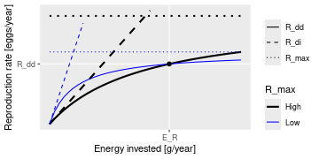
This plot shows that a given energy E_R invested into reproduction can
lead to the same reproduction rate R_{dd} with different choices
of the parameters R_max and erepro. R_max determines the asymptote of
the curve and erepro its initial slope. A higher R_max coupled with a
lower erepro (black curves) can give the same value as a lower R_max
coupled with a higher erepro (blue curves).
For the given initial state in the MizerParams object params one can
calculate the energy E_R that is invested into reproduction by the
mature individuals and the reproduction rate R_{dd} that is
required to keep the egg abundance constant. These two values determine the
location of the black dot in the above graph. You then only need one
parameter to select one curve from the family of Beverton-Holt curves going
through that point. This parameter can be erepro or R_max. Instead of
R_max you can alternatively specify the reproduction_level which is the
ratio between the density-dependent reproduction rate R_{dd} and
the maximal reproduction rate R_{max}.
If you do not provide a value for any of the reproduction parameter
arguments, then erepro will be set to the value it has in the current
species parameter data frame. If you do provide one of the reproduction
parameters, this can be either a vector with one value for each
species, or a named vector where the names determine which species are
affected, or a single unnamed value that is then used for all species. Any
species for which the given value is NA will remain unaffected.
The values for R_max must be larger than R_{dd} and can range
up to Inf. If a smaller value is requested a warning is issued and the
value is increased to the value required for a reproduction level of 0.99.
The values for the reproduction_level must be non-negative and
less than 1. The values for erepro must be large enough to allow the
required reproduction rate. If a smaller value is requested a warning is
issued and the value is increased to the smallest possible value. The values
for erepro should also be smaller than 1 to be physiologically sensible,
but this is not enforced by the function.
As can be seen in the graph above, choosing a lower value for R_max or a
higher value for erepro means that near the steady state the reproduction
will be less sensitive to a change in the energy invested into reproduction
and hence less sensitive to changes in the spawning stock biomass or its
energy income. As a result the species will also be less sensitive to
fishing, leading to a higher F_MSY.
Value
A MizerParams object
reproduction_level(): A named vector with the reproduction level
for each species.
Examples
params <- NS_params
species_params(params)$erepro
# Attempting to set the same erepro for all species
params <- setBevertonHolt(params, erepro = 0.1)
t(species_params(params)[, c("erepro", "R_max")])
# Setting erepro for some species
params <- setBevertonHolt(params, erepro = c("Gurnard" = 0.6, "Plaice" = 0.95))
t(species_params(params)[, c("erepro", "R_max")])
# Setting R_max
R_max <- 1e17 * species_params(params)$w_max^-1
params <- setBevertonHolt(NS_params, R_max = R_max)
t(species_params(params)[, c("erepro", "R_max")])
# Setting reproduction_level
params <- setBevertonHolt(params, reproduction_level = 0.3)
t(species_params(params)[, c("erepro", "R_max")])
# Inspecting reproduction level
reproduction_level(NS_params)
# The reproduction level can be changed without changing the steady state:
reproduction_level(params) <- 0.9
reproduction_level(params)
Set line colours and line types to be used in mizer plots
Description
Used for setting the colour and type of lines representing "Total",
"Resource", "Fishing", "Background", "External" and possibly other categories
in plots.
Usage
setColours(params, colours)
getColours(params)
setLinetypes(params, linetypes)
getLinetypes(params)
Arguments
params |
A MizerParams object |
colours |
A named list or named vector of line colours. |
linetypes |
A named list or named vector of linetypes. |
Details
Colours for names that already had a colour set for them will be overwritten by the colour you specify. Colours for names that did not yet have a colour will be appended to the list of colours.
If a name coincides with the name of a species, the linecolour (for
setColours()) or linetype (for setLinetypes()) entry for that species
in species_params and given_species_params is updated as well, so that
the choice persists with the species. Alternatively you can set the
linecolour and linetype variables in the species parameter data frame
directly, see the example below.
You can use the same colours in your own ggplot2 plots by adding
scale_colour_manual(values = getColours(params)) to your plot. Similarly
you can use the linetypes with
scale_linetype_manual(values = getLinetypes(params)).
Value
setColours: The MizerParams object with updated line colours
getColours(): A named vector of colours
setLinetypes(): The MizerParams object with updated linetypes
getLinetypes(): A named vector of linetypes
Examples
params <- setColours(NS_params, list("Resource" = "red","Total" = "#0000ff"))
params <- setLinetypes(NS_params, list("Total" = "dotted"))
# Set colours and linetypes for species, either via setColours()/
# setLinetypes() or directly via the species parameter data frame
params <- setColours(params, list("Cod" = "black"))
species_params(params)["Cod", "linetype"] <- "dashed"
plotSpectra(params, total = TRUE)
getColours(params)
getLinetypes(params)
Add a dynamical ecosystem component
Description
By default, mizer models any number of size-resolved consumer species and a single size-resolved resource spectrum. Your model may require additional components, like for example detritus or carrion or multiple resources or .... This function allows you to set up such components.
Usage
setComponent(
params,
component,
initial_value,
dynamics_fun,
encounter_fun,
mort_fun,
component_params,
colour = "grey",
linetype = "solid"
)
removeComponent(params, component)
getComponent(params, component)
Arguments
params |
A MizerParams object |
component |
Name of the component of interest. If missing, a list of all components will be returned. |
initial_value |
Initial value of the component |
dynamics_fun |
Name of function to calculate value at the next time step |
encounter_fun |
Name of function to calculate contribution to encounter rate. Optional. |
mort_fun |
Name of function to calculate contribution to the mortality rate. Optional. |
component_params |
Object holding the parameters needed by the component functions. This could for example be a named list of parameters. Optional. |
colour |
Line colour to use for the component in plots. Defaults to
|
linetype |
Line type to use for the component in plots. Defaults to
|
Details
The component can be a number, a vector, an array, a list, or any other data structure you like.
If you set a component with a new name, the new component will be added
to the existing components. If you set a component with an existing name,
the initial_value and dynamics_fun are overwritten, while the optional
encounter_fun, mort_fun and component_params are only changed if the
corresponding arguments are supplied. You can remove a component with
removeComponent().
Value
The updated MizerParams object
For getComponent: A list with the entries initial_value, dynamics_fun,
encounter_fun, mort_fun, component_params for the requested
component. If the requested component does not exist, NULL is returned.
If no component argument is given, then a list of lists for all
components is returned.
See Also
"Extending mizer": guide to extending mizer
Other extension tools:
NOther(),
coerceToExtensionClass(),
initialNOther<-(),
other_mort(),
recordExtension(),
setRateFunction()
Set external diffusion rate
Description
You will usually not need to call this function directly. Instead change
the D_ext and n species parameters with
given_species_params(params) <- and let mizer recalculate the external
diffusion rate for you. Call setExtDiffusion() directly only if you want
to impose a different functional form for the size dependence of the
external diffusion rate. See vignette("guide-change-parameters")
for a full explanation of when to reach for which level of the model.
Usage
setExtDiffusion(params, ext_diffusion = NULL, reset = FALSE, ...)
ext_diffusion(params)
ext_diffusion(params) <- value
Arguments
params |
MizerParams |
ext_diffusion |
Optional. An array (species x size) holding the
external diffusion rate. If not supplied, a default is calculated from the
|
reset |
If set to TRUE, then the external diffusion rate will be reset to the value calculated from the species parameters, even if it was previously overwritten with a custom value. If set to FALSE (default) then a recalculation from the species parameters will take place only if no custom value has been set. |
... |
Unused |
value |
ext_diffusion |
Value
setExtDiffusion(): A MizerParams object with updated external
diffusion rate.
ext_diffusion(): An ArraySpeciesBySize object (species x size)
with the external diffusion rate.
Setting external diffusion rate
The external diffusion rate allows you to impose additional diffusion beyond the predation-driven diffusion that can be internally modelled by mizer.
The ext_diffusion argument allows you to specify a diffusion rate that
depends on species and body size.
If the ext_diffusion argument is not supplied, then the external diffusion
rate is calculated as a power law:
D_{ext.i}(w) = D_{ext.i}\, w^{n_i+1}.
The coefficient D_{ext.i} is taken from the D_ext column of the
species parameter data frame, which defaults to 0. The exponent
n_i + 1 uses the n column of the species parameter data frame.
If the ext_diffusion slot has a comment and reset = FALSE, then a
recalculation from the species parameters is suppressed and a message is
issued if the recalculated values would differ from the stored ones.
See Also
Other functions for setting parameters:
gear_params(),
setExtEncounter(),
setExtMort(),
setFishing(),
setInteraction(),
setMaxIntakeRate(),
setMetabolicRate(),
setParams(),
setPredKernel(),
setReproduction(),
setSearchVolume(),
species_params(),
use_predation_diffusion()
Set external encounter rate
Description
You will usually not need to call this function directly. Instead change
the E_ext and n species parameters with
given_species_params(params) <- and let mizer recalculate the external
encounter rate for you. Call setExtEncounter() directly only if you want
to impose a different functional form for the size dependence of the
external encounter rate. See vignette("guide-change-parameters")
for a full explanation of when to reach for which level of the model.
Usage
setExtEncounter(params, ext_encounter = NULL, reset = FALSE, ...)
ext_encounter(params)
ext_encounter(params) <- value
Arguments
params |
MizerParams |
ext_encounter |
Optional. An array (species x size) holding the external
encounter rate. If not supplied, a default is calculated from the |
reset |
If set to TRUE, then the external encounter rate will be reset to the value calculated from the species parameters, even if it was previously overwritten with a custom value. If set to FALSE (default) then a recalculation from the species parameters will take place only if no custom value has been set. |
... |
Unused |
value |
ext_encounter |
Value
setExtEncounter(): A MizerParams object with updated external encounter
rate.
ext_encounter(): An ArraySpeciesBySize object (species x size)
with the external encounter rate.
Setting external encounter rate
The external encounter rate is the rate at which a predator encounters food that is not explicitly modelled. It is a rate with units mass/year.
The ext_encounter argument allows you to specify an external encounter rate
that depends on species and body size. You can see an example of this in
the Examples section of the help page for setExtEncounter().
If the ext_encounter argument is not supplied, then the external encounter
rate is calculated as a power law:
E_{ext.i}(w) = E_{ext.i}\, w^{n_i}.
The coefficient E_{ext.i} is taken from the E_ext column of the
species parameter data frame, which defaults to 0. The exponent n_i is
taken from the n column of the species parameter data frame.
If the ext_encounter slot has a comment and reset = FALSE, then a
recalculation from the species parameters is suppressed and a message is
issued if the recalculated values would differ from the stored ones.
See Also
Other functions for setting parameters:
gear_params(),
setExtDiffusion(),
setExtMort(),
setFishing(),
setInteraction(),
setMaxIntakeRate(),
setMetabolicRate(),
setParams(),
setPredKernel(),
setReproduction(),
setSearchVolume(),
species_params(),
use_predation_diffusion()
Examples
params <- newMultispeciesParams(NS_species_params)
#### Setting allometric encounter rate #######################
# Set coefficient for each species. Here we choose 0.1 for each species
encounter_pre <- rep(0.1, nrow(species_params(params)))
# Multiply by power of size with exponent, here chosen to be 3/4
# The outer() function makes it an array species x size
allo_encounter <- outer(encounter_pre, w(params)^(3/4))
# Change the external encounter rate in the params object
ext_encounter(params) <- allo_encounter
Set external mortality rate
Description
You will usually not need to call this function directly. Instead change
the z0, z_ext and d species parameters with
given_species_params(params) <- and let mizer recalculate the external
mortality rate for you. Call setExtMort() directly only if you want to
impose a different functional form for the size dependence of the external
mortality. See vignette("guide-change-parameters") for a full
explanation of when to reach for which level of the model.
Usage
setExtMort(
params,
ext_mort = NULL,
z0pre = 0.6,
z0exp = params@resource_params$n - 1,
reset = FALSE,
z0 = deprecated(),
...
)
ext_mort(params)
ext_mort(params) <- value
Arguments
params |
MizerParams |
ext_mort |
Optional. An array (species x size) holding the external mortality rate. If not supplied, a default is set as described in the section "Setting external mortality rate". |
z0pre |
If |
z0exp |
The exponent used with |
reset |
If set to TRUE, then the external mortality rate will be reset to the value calculated from the species parameters, even if it was previously overwritten with a custom value. If set to FALSE (default) then a recalculation from the species parameters will take place only if no custom value has been set. |
z0 |
|
... |
Unused |
value |
ext_mort |
Value
setExtMort(): A MizerParams object with updated external mortality
rate.
ext_mort(): An ArraySpeciesBySize object (species x size) with
the external mortality.
Setting external mortality rate
The external mortality is all the mortality that is not due to fishing or predation by predators included in the model. The external mortality could be due to predation by predators that are not explicitly included in the model (e.g. mammals or seabirds) or due to other causes like illness. It is a rate with units 1/year.
The ext_mort argument allows you to specify an external mortality rate
that depends on species and body size. You can see an example of this in
the Examples section of the help page for setExtMort().
If the ext_mort argument is not supplied, then the external mortality is
taken from the species parameters as
\mu_{ext.i}(w) = z_{0.i} + z_{ext.i} w^{d_i}.
The value of the constant z_0 for each species is taken from the z0
column of given_species_params() if it is present there. Otherwise it is
recalculated, even if a value from an earlier calculation is still present
in species_params, as
z_{0.i} = {\tt z0pre}_i\, w_{inf}^{\tt z0exp}.
When z0pre or z0exp is supplied explicitly and used to calculate
non-given z0, the resulting values are recorded in
given_species_params(). Values calculated from the defaults
z0pre = 0.6 and z0exp = n - 1 are not recorded there. If either argument
is supplied but cannot be used because z0 is given for every species or
because ext_mort was supplied, a warning is issued.
Missing values of z_ext are set to 0 and missing values of d are set to
n - 1.
By default the power law is evaluated at the left bin edges w_j
(point sampling). If the bin_average entry of the second_order_w slot is
TRUE (see second_order_w()), then the z_{ext} w^d term is instead
replaced by its exact average over each bin [w_j, w_{j+1}],
\frac{z_{ext}}{\Delta w_j}\int_{w_j}^{w_{j+1}} w^d\, dw
= z_{ext}\,\frac{w_{j+1}^{d+1} - w_j^{d+1}}{(d+1)\,\Delta w_j},
(with the limiting form z_{ext}\ln(w_{j+1}/w_j)/\Delta w_j when
d = -1). This is the consistent choice in the finite-volume scheme,
where the external mortality multiplies the bin-averaged abundance. The
bin-averaging is applied only to the auto-calculated power-law default; a
user-supplied ext_mort array is left untouched.
See Also
Other functions for setting parameters:
gear_params(),
setExtDiffusion(),
setExtEncounter(),
setFishing(),
setInteraction(),
setMaxIntakeRate(),
setMetabolicRate(),
setParams(),
setPredKernel(),
setReproduction(),
setSearchVolume(),
species_params(),
use_predation_diffusion()
Examples
params <- newMultispeciesParams(NS_species_params)
#### Setting allometric death rate #######################
# Set coefficient for each species. Here we choose 0.1 for each species
z0pre <- rep(0.1, nrow(species_params(params)))
# Multiply by power of size with exponent, here chosen to be -1/4
# The outer() function makes it an array species x size
allo_mort <- outer(z0pre, w(params)^(-1/4))
# Change the external mortality rate in the params object
ext_mort(params) <- allo_mort
Set fishing parameters
Description
Set fishing parameters
Usage
setFishing(
params,
selectivity = NULL,
catchability = NULL,
reset = FALSE,
initial_effort = NULL,
...
)
catchability(params)
catchability(params) <- value
selectivity(params)
selectivity(params) <- value
Arguments
params |
A MizerParams object |
selectivity |
Optional. An array (gear x species x size) that holds the
selectivity of each gear for species and size, |
catchability |
Optional. An array (gear x species) that holds the catchability of
each species by each gear, |
reset |
If set to TRUE, then both |
initial_effort |
Optional. A number or a named numeric vector specifying the fishing effort. If a number, the same effort is used for all gears. If a vector, must be named by gear. |
... |
Unused |
value |
The array to assign |
Value
setFishing(): A MizerParams object with updated fishing
parameters.
catchability(): An array (gear x species) that holds the
catchability of each species by each gear,
Q_{g,i}. The names of the dimensions are "gear, "sp".
selectivity(): An array (gear x species x size) that holds the
selectivity of each gear for species and
size, S_{g,i,w}. The names of the dimensions are "gear, "sp", "w".
Setting fishing
Gears
In mizer, fishing mortality is imposed on species by fishing gears. The
total per-capita fishing mortality (1/year) is obtained by summing over the
mortality from all gears,
\mu_{f.i}(w) = \sum_g F_{g,i}(w),
where the fishing mortality F_{g,i}(w) imposed by gear g on
species i at size w is calculated as:
F_{g,i}(w) = S_{g,i}(w) Q_{g,i} E_{g},
where S is the selectivity by species, gear and size, Q is the
catchability by species and gear and E is the fishing effort by gear.
Selectivity
The selectivity at size of each gear for each species is saved as a three
dimensional array (gear x species x size). Each entry has a range between 0
(that gear is not selecting that species at that size) to 1 (that gear is
selecting all individuals of that species of that size). This three
dimensional array can be specified explicitly via the selectivity
argument, but usually mizer calculates it from the gear_params slot of
the MizerParams object.
To allow the calculation of the selectivity array, the gear_params slot
must be a data frame with one row for each gear-species combination. So if
for example a gear can select three species, then that gear contributes three
rows to the gear_params data frame, one for each species it can select. The
data frame must have columns gear, holding the name of the gear, species,
holding the name of the species, and sel_func, holding the name of the
function that calculates the selectivity curve. Some selectivity functions
are included in the package: knife_edge(), sigmoid_length(),
double_sigmoid_length(), and sigmoid_weight().
Users are able to write their own size-based selectivity function. The first
argument to the function must be w and the function must return a vector of
the selectivity (between 0 and 1) at size.
Each selectivity function may have parameters. Values for these
parameters must be included as columns in the gear parameters data.frame.
The names of the columns must exactly match the names of the corresponding
arguments of the selectivity function. For example, the default selectivity
function is knife_edge() that a has sudden change of selectivity from 0 to 1
at a certain size. In its help page you can see that the knife_edge()
function has arguments w and knife_edge_size. The first argument, w, is
size (the function calculates selectivity at size). All selectivity functions
must have w as the first argument. The values for the other arguments must
be found in the gear parameters data.frame. So for the knife_edge()
function there should be a knife_edge_size column. Because knife_edge()
is the default selectivity function, the knife_edge_size argument has a
default value = w_mat.
The most commonly-used selectivity function is sigmoid_length(). It has a
smooth transition from 0 to 1 at a certain size. The sigmoid_length()
function has the two parameters l50 and l25 that are the lengths in cm at
which 50% or 25% of the fish are selected by the gear. If you choose this
selectivity function then the l50 and l25 columns must be included in the
gear parameters data.frame.
In case each species is only selected by one gear, the columns of the
gear_params data frame can alternatively be provided as columns of the
species_params data frame, if this is more convenient for the user to set
up. Mizer will then copy these columns over to create the gear_params data
frame when it creates the MizerParams object. However changing these columns
in the species parameter data frame later will not update the gear_params
data frame.
Catchability
Catchability is used as an additional factor to make the link between gear selectivity, fishing effort and fishing mortality. For example, it can be set so that an effort of 1 gives a desired fishing mortality. In this way effort can then be specified relative to a 'base effort', e.g. the effort in a particular year.
Catchability is stored as a two dimensional array (gear x species). This can
either be provided explicitly via the catchability argument, or the
information can be provided via a catchability column in the gear_params
data frame.
In the case where each species is selected by only a single gear, the
catchability column can also be provided in the species_params data
frame. Mizer will then copy this over to the gear_params data frame when
the MizerParams object is created.
Effort
The initial fishing effort is stored in the MizerParams object. If it is
not supplied, it is set to zero. The initial effort can be overruled when
the simulation is run with project(), where it is also possible to specify
an effort that varies through time.
See Also
Other functions for setting parameters:
gear_params(),
setExtDiffusion(),
setExtEncounter(),
setExtMort(),
setInteraction(),
setMaxIntakeRate(),
setMetabolicRate(),
setParams(),
setPredKernel(),
setReproduction(),
setSearchVolume(),
species_params(),
use_predation_diffusion()
Examples
# Halve the initial fishing effort for all gears
params <- setFishing(NS_params, initial_effort = 0.5)
initial_effort(params)
str(catchability(NS_params))
str(selectivity(NS_params))
Set initial values to values from a simulation
Description
This function is deprecated. Use getParams(), initialParams(), or
finalParams() instead. These functions return a MizerParams object
with the ecosystem state extracted from a simulation.
Usage
setInitialValues(params, sim, time_range, geometric_mean = FALSE, ...)
Arguments
params |
A |
sim |
A |
time_range |
The time range to average the abundances over. Can be a vector of values, a vector of min and max time, or a single value. Only the range of times is relevant, i.e., all times between the smallest and largest will be selected. Default is the final time step. |
geometric_mean |
|
... |
Additional arguments passed to the method. |
Details
Value
The params object with updated initial values and initial effort.
Examples
params <- NS_params
sim <- project(params, t_max = 20, effort = 0.5)
params <- setInitialValues(params, sim)
Set species interaction matrix
Description
Set species interaction matrix
Usage
setInteraction(params, interaction = NULL, ...)
interaction_matrix(params)
interaction_matrix(params) <- value
Arguments
params |
MizerParams object |
interaction |
Optional interaction matrix of the species (predator species x prey species). By default all entries are 1. See "Setting interaction matrix" section below. |
... |
Unused |
value |
An interaction matrix |
Value
setInteraction: A MizerParams object with updated interaction
matrix
interaction_matrix(): The interaction matrix (predator species x
prey species)
Setting interaction matrix
You do not need to specify an interaction matrix. If you do not, then the predator-prey interactions are purely determined by the size of predator and prey and totally independent of the species of predator and prey.
The interaction matrix \theta_{ij} modifies the interaction of each
pair of species in the model. This can be used for example to allow for
different spatial overlap among the species.
The values in the interaction matrix are used to scale the encountered food
and predation mortality (see on the website the section on predator-prey encounter rate
and on predation mortality).
The first index refers to the predator species and the second to the prey
species.
The interaction matrix is used when calculating the food encounter rate in
getEncounter() and the predation mortality rate in getPredMort(). Its
entries are dimensionless numbers. If all the values in the interaction
matrix are equal then predator-prey interactions are determined entirely by
size-preference.
This function checks that the supplied interaction matrix is valid and then
stores it in the interaction slot of the params object.
The order of the columns and rows of the interaction argument should be
the same as the order in the species params data frame in the params
object. If you supply a named array then the function will check the order
and message if it is different before ignoring the supplied dimnames. If
you supply only column names then these are also used as the row names. One
way of creating your own interaction
matrix is to enter the data using a spreadsheet program and saving it as a
.csv file. The data can then be read into R using the command read.csv().
The interaction of the species with the resource are set via a column
interaction_resource in the species_params data frame. By default this
column is set to all 1s.
See Also
Other functions for setting parameters:
gear_params(),
setExtDiffusion(),
setExtEncounter(),
setExtMort(),
setFishing(),
setMaxIntakeRate(),
setMetabolicRate(),
setParams(),
setPredKernel(),
setReproduction(),
setSearchVolume(),
species_params(),
use_predation_diffusion()
Examples
params <- newTraitParams(no_sp = 3)
inter <- interaction_matrix(params)
inter[1, 2:3] <- 0
params <- setInteraction(params, interaction = inter)
interaction_matrix(params)
Set maximum intake rate
Description
You will usually not need to call this function directly. Instead change
the h and n species parameters with given_species_params(params) <-
and let mizer recalculate the maximum intake rate for you. Call
setMaxIntakeRate() directly only if you want to impose a different
functional form for the size dependence of the intake rate. See
vignette("guide-change-parameters") for a full explanation of when
to reach for which level of the model.
Usage
setMaxIntakeRate(params, intake_max = NULL, reset = FALSE, ...)
intake_max(params)
intake_max(params) <- value
Arguments
params |
MizerParams |
intake_max |
Optional. An array (species x size) holding the maximum intake rate for each species at size. If not supplied, a default is set as described in the section "Setting maximum intake rate". |
reset |
If set to TRUE, then the intake rate will be reset to the value calculated from the species parameters, even if it was previously overwritten with a custom value. If set to FALSE (default) then a recalculation from the species parameters will take place only if no custom value has been set. |
... |
Unused |
value |
intake_max |
Value
setMaxIntakeRate(): A MizerParams object with updated maximum
intake rate.
intake_max(): An ArraySpeciesBySize object (species x size) with
the maximum intake rate.
Setting maximum intake rate
The maximum intake rate h_i(w) of an individual of species i and
weight w determines the feeding level, calculated with
getFeedingLevel(). It is measured in grams/year.
If the intake_max argument is not supplied, then the maximum intake
rate is set to
h_i(w) = h_i w^{n_i}.
The values of h_i (the maximum intake rate of an individual of size 1
gram) and n_i (the allometric exponent for the intake rate) are taken
from the h and n columns in the species parameter dataframe. If
the h column is not supplied in the species parameter dataframe, it is
calculated by the get_h_default() function. If the n column is not
supplied, a default of n_i = 3/4 is used.
If h_i is set to Inf, fish of species i will consume all encountered
food.
If the intake_max slot has a comment and reset = FALSE, then a
recalculation from the species parameters is suppressed and a message is
issued if the recalculated values would differ from the stored ones.
See Also
Other functions for setting parameters:
gear_params(),
setExtDiffusion(),
setExtEncounter(),
setExtMort(),
setFishing(),
setInteraction(),
setMetabolicRate(),
setParams(),
setPredKernel(),
setReproduction(),
setSearchVolume(),
species_params(),
use_predation_diffusion()
Examples
# Inspect the current maximum intake rate
intake_max(NS_params)["Cod", 1:5]
# Increase intake rate for Cod by 50%
im <- intake_max(NS_params)
im["Cod", ] <- im["Cod", ] * 1.5
params <- setMaxIntakeRate(NS_params, intake_max = im)
intake_max(params)["Cod", 1:5]
Set metabolic rate
Description
Sets the rate at which energy is used for metabolism and activity. You will
usually not need to call this function directly. Instead change the k,
ks and p species parameters with given_species_params(params) <- and
let mizer recalculate the metabolic rate for you. Call setMetabolicRate()
directly only if you want to impose a different functional form for the
size dependence of the metabolic rate. See
vignette("guide-change-parameters") for a full explanation of when
to reach for which level of the model.
Usage
setMetabolicRate(object, metab = NULL, p = deprecated(), reset = FALSE, ...)
metab(params)
metab(params) <- value
Arguments
object |
A MizerParams object |
metab |
Optional. An array (species x size) holding the metabolic rate for each species at size. If not supplied, a default is set as described in the section "Setting metabolic rate". |
p |
|
reset |
If set to TRUE, then the metabolic rate will be reset to the value calculated from the species parameters, even if it was previously overwritten with a custom value. If set to FALSE (default) then a recalculation from the species parameters will take place only if no custom value has been set. |
... |
Unused |
params |
A MizerParams object |
value |
metab |
Value
setMetabolicRate(): A MizerParams object with updated metabolic rate.
metab(): An ArraySpeciesBySize object (species x size) with the
metabolic rate.
Setting metabolic rate
The metabolic rate is subtracted from the energy income rate to calculate
the rate at which energy is available for growth and reproduction, see
getEReproAndGrowth(). It is measured in grams/year.
If the metab argument is not supplied, then for each species the
metabolic rate k(w) for an individual of size w is set to
k(w) = k_s w^p + k w,
where k_s w^p represents the rate of standard metabolism and k w
is the rate at which energy is expended on activity and movement. The values
of k_s, p and k are taken from the ks, p and
k columns in the species parameter dataframe. If any of these
parameters are not supplied, the defaults are k = 0, p = n and
k_s = f_c h \alpha w_{mat}^{n-p},
where f_c is the critical feeding level taken from the fc column
in the species parameter data frame. If the critical feeding level is not
specified, a default of f_c = 0.2 is used.
If the metab slot has a comment and reset = FALSE, then a recalculation
from the species parameters is suppressed and a message is issued if the
recalculated values would differ from the stored ones.
See Also
Other functions for setting parameters:
gear_params(),
setExtDiffusion(),
setExtEncounter(),
setExtMort(),
setFishing(),
setInteraction(),
setMaxIntakeRate(),
setParams(),
setPredKernel(),
setReproduction(),
setSearchVolume(),
species_params(),
use_predation_diffusion()
Examples
# Inspect the current metabolic rate
metab(NS_params)["Cod", 1:5]
# Reset metabolic rate from species parameters
params <- setMetabolicRate(NS_params, reset = TRUE)
metab(params)["Cod", 1:5]
Set metadata for a model
Description
Setting metadata is particularly important for sharing your model with others. All metadata fields are optional and you can also add other fields of your own choosing. If you set a value for a field that already existed, the old value will be overwritten.
Usage
setMetadata(
params,
title = NULL,
description = NULL,
authors = NULL,
url = NULL,
doi = NULL,
...
)
getMetadata(params)
Arguments
params |
The MizerParams object for the model |
title |
A string with the title for the model |
description |
A string with a description of the model. This could for example contain information about any publications using the model. |
authors |
An author entry or a list of author entries, where each author
entry could either be just a name or could itself be a list with fields
like |
url |
A URL where more information about the model can be found. This could be a blog post on the mizer blog, for example. |
doi |
The digital object identifier for your model. To create a doi you can use online services like https://zenodo.org/ or https://figshare.com. |
... |
Additional metadata fields that you would like to add |
Details
In addition to the metadata fields you can set by hand, there are four fields that are set automatically by mizer:
-
mizer_versionThe version string of the mizer version under which the model was created or last upgraded. Can be compared to the current version which is obtained withpackageVersion("mizer"). The purpose of this field is that if the model is not working as expected in the current version of mizer, you can go back to the older version under which presumably it was working. -
extensionsA named list with one entry for each extension package needed to run the model. Each entry records the installationrequirementand the packageversionwhose object layout is in use. This field is set by extension packages withrecordExtension()and can be inspected withgetMetadata(params)$extensions. -
time_createdA POSIXct date-time object with the creation time. -
time_modifiedA POSIXct date-time object with the last modified time.
Setting the metadata with this function does not count as a modification of
the object, so the time_modified field will not be updated.
Value
setMetadata(): The MizerParams object with updated metadata
getMetadata(): A list with all metadata entries that have been set,
including at least
mizer_version, extensions, time_created and time_modified.
Examples
params <- setMetadata(NS_params,
title = "North Sea model",
description = "A multi-species model of the North Sea fish community.",
authors = list(list(name = "Finlay Scott", email = "finlay@example.com")),
my_own_filed = "something that doesn't fit elsewhere")
getMetadata(params)$title
getMetadata(params)$authors[[1]]$name
Set or change any model parameters
Description
This is a convenient wrapper function calling each of the following functions
Note that setResource() is not among them: the resource rate, capacity
and dynamics are not changed by setParams() and have to be set with
setResource(). Passing a resource argument to setParams() gives an error
rather than being silently ignored. See the Details section below for a
discussion of how to use this function.
Usage
setParams(
object,
interaction = NULL,
info_level = default_info_level(),
...,
reset = FALSE
)
Arguments
object |
A MizerParams object |
interaction |
Optional interaction matrix of the species (predator species x prey species). By default all entries are 1. See "Setting interaction matrix" section below. |
info_level |
Controls the amount of information messages that are shown.
Higher levels lead to more messages, |
... |
Arguments passed on to
|
reset |
If set to TRUE then all the rate arrays that |
Details
If you are not happy with the assumptions that mizer makes by default about
the size-dependence of parameters, for example if you want to change one of
the allometric scaling assumptions, you can do this by providing your
choice as an array in the appropriate argument to setParams(). The
sections below discuss all the model functions that you can change this way.
Because of the way the R language works, setParams does not make the
changes to the params object that you pass to it but instead returns a new
params object. So to affect the change you call the function in the form
params <- setParams(params, ...).
Usually, if you are happy with the way mizer calculates the size-dependent parameters
from the species parameters and only want to change the values of some
species parameters, you would make those changes in the species_params data
frame contained in the params object using species_params<-().
Here is an example which assumes that
you have have a MizerParams object params in which you just want to change
the gamma parameter of the third species:
species_params(params)$gamma[[3]] <- 1000
Internally that will actually call setParams() to recalculate any of the
other parameters that are affected by the change in the species parameter.
setParams() will use the species parameters in the params object to
recalculate the values of all the parameter arrays except those for which you
have set custom values.
Value
A MizerParams object
Units in mizer
Mizer uses grams to measure weight, centimetres to measure lengths, and years to measure time.
Mizer is agnostic about whether abundances are given as
numbers per area,
numbers per volume or
total numbers for the entire study area.
You should make the choice most convenient for your application and then stick with it. If you make choice 1 or 2 you will also have to choose a unit for area or volume. Your choice will then determine the units for some of the parameters. This will be mentioned when the parameters are discussed in the sections below.
Your choice will also affect the units of the quantities you may want to
calculate with the model. For example, the yield will be in grams/year/m^2 in
case 1 if you choose m^2 as your measure of area, in grams/year/m^3 in case 2
if you choose m^3 as your unit of volume, or simply grams/year in case 3. The
same comment applies for other measures, like total biomass, which will be
grams/area in case 1, grams/volume in case 2 or simply grams in case 3. When
mizer puts units on axes in plots, it will choose the units appropriate for
case 3. So for example in plotBiomass() it gives the unit as grams.
You can convert between these choices. For example, if you use case 1, you
need to multiply with the area of the ecosystem to get the total quantity.
If you work with case 2, you need to multiply by both area and the thickness
of the productive layer. In that respect, case 2 is a bit cumbersome. The
function scaleModel() is useful to change the units you are using.
Setting interaction matrix
You do not need to specify an interaction matrix. If you do not, then the predator-prey interactions are purely determined by the size of predator and prey and totally independent of the species of predator and prey.
The interaction matrix \theta_{ij} modifies the interaction of each
pair of species in the model. This can be used for example to allow for
different spatial overlap among the species.
The values in the interaction matrix are used to scale the encountered food
and predation mortality (see on the website the section on predator-prey encounter rate
and on predation mortality).
The first index refers to the predator species and the second to the prey
species.
The interaction matrix is used when calculating the food encounter rate in
getEncounter() and the predation mortality rate in getPredMort(). Its
entries are dimensionless numbers. If all the values in the interaction
matrix are equal then predator-prey interactions are determined entirely by
size-preference.
This function checks that the supplied interaction matrix is valid and then
stores it in the interaction slot of the params object.
The order of the columns and rows of the interaction argument should be
the same as the order in the species params data frame in the params
object. If you supply a named array then the function will check the order
and message if it is different before ignoring the supplied dimnames. If
you supply only column names then these are also used as the row names. One
way of creating your own interaction
matrix is to enter the data using a spreadsheet program and saving it as a
.csv file. The data can then be read into R using the command read.csv().
The interaction of the species with the resource are set via a column
interaction_resource in the species_params data frame. By default this
column is set to all 1s.
Setting predation kernel
Kernel dependent on predator to prey size ratio
If the pred_kernel argument is not supplied, then this function sets a
predation kernel that depends only on the ratio of predator mass to prey
mass, not on the two masses independently. The shape of that kernel is then
determined by the pred_kernel_type column in species_params.
The default for pred_kernel_type is "lognormal". This will call the function
lognormal_pred_kernel() to calculate the predation kernel.
Alternative pred_kernel types are "box", implemented by box_pred_kernel(),
"power_law", implemented by power_law_pred_kernel(), and
"gaussian_mixture", implemented by gaussian_mixture_pred_kernel(). These
functions require certain species parameters in the species_params data
frame. For the lognormal kernel these are beta and sigma, for the box
kernel they are ppmr_min and ppmr_max, and for the Gaussian mixture they
are the list-columns kernel_p, kernel_mean, and kernel_sd. They are
explained in the help pages for the kernel functions. Except for beta and
sigma, no defaults are set for these parameters. If they are missing from
the species_params data frame then mizer will issue an error message.
You can use any other string for pred_kernel_type. If for example you
choose "my" then you need to define a function my_pred_kernel that you can
model on the existing functions like lognormal_pred_kernel().
When using a kernel that depends on the predator/prey size ratio only, mizer
does not need to store the entire three dimensional array in the MizerParams
object. Such an array can be very big when there is a large number of size
bins. Instead, mizer only needs to store two two-dimensional arrays that hold
Fourier transforms of the feeding kernel function that allow the encounter
rate and the predation rate to be calculated very efficiently. However, if
you need the full three-dimensional array you can calculate it with the
pred_kernel() function.
Kernel dependent on both predator and prey size
If you want to work with a feeding kernel that depends on predator mass and prey mass independently, you can specify the full feeding kernel as a three-dimensional array (predator species x predator size x prey size).
You should use this option only if a kernel dependent only on the predator/prey mass ratio is not appropriate. Using a kernel dependent on predator/prey mass ratio only allows mizer to use fast Fourier transform methods to significantly reduce the running time of simulations.
The order of the predator species in pred_kernel should be the same
as the order in the species params dataframe in the params object. If you
supply a named array then the function will check the order and warn if it is
different.
Setting search volume
The search volume \gamma_i(w) of an individual of species i
and weight w multiplies the predation kernel when
calculating the encounter rate in getEncounter() and the
predation rate in getPredRate().
The name "search volume" is a bit misleading, because \gamma_i(w) does
not have units of volume. It is simply a parameter that determines the rate
of predation. Its units depend on your choice, see section "Units in mizer".
If you have chosen to work with total abundances, then it is a rate with units
1/year. If you have chosen to work with abundances per m^2 then it has units
of m^2/year. If you have chosen to work with abundances per m^3 then it has
units of m^3/year.
If the search_vol argument is not supplied, then the search volume is
set to
\gamma_i(w) = \gamma_i w^q_i.
The values of \gamma_i (the search volume at 1g) and q_i (the
allometric exponent of the search volume) are taken from the gamma and
q columns in the species parameter dataframe. If the gamma
column is not supplied in the species parameter dataframe, a default is
calculated by the get_gamma_default() function. If the q column is not
supplied, a default of lambda - 2 + n is used. Note that only
for predators of size w = 1 gram is the value of the species parameter
\gamma_i the same as the value of the search volume \gamma_i(w).
If the search_vol slot has a comment and reset = FALSE, then a
recalculation from the species parameters is suppressed and a message is
issued if the recalculated values would differ from the stored ones.
Setting maximum intake rate
The maximum intake rate h_i(w) of an individual of species i and
weight w determines the feeding level, calculated with
getFeedingLevel(). It is measured in grams/year.
If the intake_max argument is not supplied, then the maximum intake
rate is set to
h_i(w) = h_i w^{n_i}.
The values of h_i (the maximum intake rate of an individual of size 1
gram) and n_i (the allometric exponent for the intake rate) are taken
from the h and n columns in the species parameter dataframe. If
the h column is not supplied in the species parameter dataframe, it is
calculated by the get_h_default() function. If the n column is not
supplied, a default of n_i = 3/4 is used.
If h_i is set to Inf, fish of species i will consume all encountered
food.
If the intake_max slot has a comment and reset = FALSE, then a
recalculation from the species parameters is suppressed and a message is
issued if the recalculated values would differ from the stored ones.
Setting metabolic rate
The metabolic rate is subtracted from the energy income rate to calculate
the rate at which energy is available for growth and reproduction, see
getEReproAndGrowth(). It is measured in grams/year.
If the metab argument is not supplied, then for each species the
metabolic rate k(w) for an individual of size w is set to
k(w) = k_s w^p + k w,
where k_s w^p represents the rate of standard metabolism and k w
is the rate at which energy is expended on activity and movement. The values
of k_s, p and k are taken from the ks, p and
k columns in the species parameter dataframe. If any of these
parameters are not supplied, the defaults are k = 0, p = n and
k_s = f_c h \alpha w_{mat}^{n-p},
where f_c is the critical feeding level taken from the fc column
in the species parameter data frame. If the critical feeding level is not
specified, a default of f_c = 0.2 is used.
If the metab slot has a comment and reset = FALSE, then a recalculation
from the species parameters is suppressed and a message is issued if the
recalculated values would differ from the stored ones.
Setting external mortality rate
The external mortality is all the mortality that is not due to fishing or predation by predators included in the model. The external mortality could be due to predation by predators that are not explicitly included in the model (e.g. mammals or seabirds) or due to other causes like illness. It is a rate with units 1/year.
The ext_mort argument allows you to specify an external mortality rate
that depends on species and body size. You can see an example of this in
the Examples section of the help page for setExtMort().
If the ext_mort argument is not supplied, then the external mortality is
taken from the species parameters as
\mu_{ext.i}(w) = z_{0.i} + z_{ext.i} w^{d_i}.
The value of the constant z_0 for each species is taken from the z0
column of given_species_params() if it is present there. Otherwise it is
recalculated, even if a value from an earlier calculation is still present
in species_params, as
z_{0.i} = {\tt z0pre}_i\, w_{inf}^{\tt z0exp}.
When z0pre or z0exp is supplied explicitly and used to calculate
non-given z0, the resulting values are recorded in
given_species_params(). Values calculated from the defaults
z0pre = 0.6 and z0exp = n - 1 are not recorded there. If either argument
is supplied but cannot be used because z0 is given for every species or
because ext_mort was supplied, a warning is issued.
Missing values of z_ext are set to 0 and missing values of d are set to
n - 1.
By default the power law is evaluated at the left bin edges w_j
(point sampling). If the bin_average entry of the second_order_w slot is
TRUE (see second_order_w()), then the z_{ext} w^d term is instead
replaced by its exact average over each bin [w_j, w_{j+1}],
\frac{z_{ext}}{\Delta w_j}\int_{w_j}^{w_{j+1}} w^d\, dw
= z_{ext}\,\frac{w_{j+1}^{d+1} - w_j^{d+1}}{(d+1)\,\Delta w_j},
(with the limiting form z_{ext}\ln(w_{j+1}/w_j)/\Delta w_j when
d = -1). This is the consistent choice in the finite-volume scheme,
where the external mortality multiplies the bin-averaged abundance. The
bin-averaging is applied only to the auto-calculated power-law default; a
user-supplied ext_mort array is left untouched.
Setting external encounter rate
The external encounter rate is the rate at which a predator encounters food that is not explicitly modelled. It is a rate with units mass/year.
The ext_encounter argument allows you to specify an external encounter rate
that depends on species and body size. You can see an example of this in
the Examples section of the help page for setExtEncounter().
If the ext_encounter argument is not supplied, then the external encounter
rate is calculated as a power law:
E_{ext.i}(w) = E_{ext.i}\, w^{n_i}.
The coefficient E_{ext.i} is taken from the E_ext column of the
species parameter data frame, which defaults to 0. The exponent n_i is
taken from the n column of the species parameter data frame.
If the ext_encounter slot has a comment and reset = FALSE, then a
recalculation from the species parameters is suppressed and a message is
issued if the recalculated values would differ from the stored ones.
Setting external diffusion rate
The external diffusion rate allows you to impose additional diffusion beyond the predation-driven diffusion that can be internally modelled by mizer.
The ext_diffusion argument allows you to specify a diffusion rate that
depends on species and body size.
If the ext_diffusion argument is not supplied, then the external diffusion
rate is calculated as a power law:
D_{ext.i}(w) = D_{ext.i}\, w^{n_i+1}.
The coefficient D_{ext.i} is taken from the D_ext column of the
species parameter data frame, which defaults to 0. The exponent
n_i + 1 uses the n column of the species parameter data frame.
If the ext_diffusion slot has a comment and reset = FALSE, then a
recalculation from the species parameters is suppressed and a message is
issued if the recalculated values would differ from the stored ones.
Setting reproduction
For each species and at each size, the proportion \psi of the
available energy
that is invested into reproduction is the product of two factors: the
proportion maturity of individuals that are mature and the proportion
repro_prop of the energy available to a mature individual that is
invested into reproduction. There is a size w_repro_max at which a typical
mature individual invests all of its available energy into reproduction.
This is not a hard ceiling on size: not all individuals are mature at
w_repro_max, and diffusion in the growth process allows some individuals to
grow beyond it, so fish larger than w_repro_max can exist. If you have not
specified the w_repro_max column in the species parameter data frame, then
the von Bertalanffy asymptotic size w_inf is used instead.
Maturity ogive
If the the proportion of individuals that are mature is not supplied via
the maturity argument, then it is set to a sigmoidal
maturity ogive that changes from 0 to 1 at around the maturity size:
{\tt maturity}(w) = \left[1+\left(\frac{w}{w_{mat}}\right)^{-U}\right]^{-1}.
(To avoid clutter, we are not showing the species index in the equations,
although each species has its own maturity ogive.)
The maturity weights are taken from the w_mat column of the
species_params data frame. Any missing maturity weights are set to 1/4 of the
asymptotic size in the w_inf column.
The exponent U determines the steepness of the maturity ogive. By
default it is chosen as U = 10, however this can be overridden by
including a column w_mat25 in the species parameter dataframe that
specifies the weight at which 25% of individuals are mature, which sets
U = \log(3) / \log(w_{mat} / w_{mat25}).
The sigmoidal function given above would strictly reach 0 only
asymptotically and thus have some (negligible) amount of reproduction at
arbitrarily small size.
For computational simplicity, any proportion smaller than
1e-8 is set to 0.
Investment into reproduction
If the the energy available to a mature individual that is
invested into reproduction is not supplied via the repro_prop argument,
it is set to the allometric form
{\tt repro\_prop}(w) =
\min\left(\left(\dfrac{w}{w_{\tt{repro\_max}}}\right)^{m-n},1\right).
Here n is the scaling exponent of the energy income rate. Hence
the exponent m determines the scaling of the investment into
reproduction for mature individuals. By default it is chosen to be
m = 1 so that the rate at which energy is invested into reproduction
scales linearly with the size. This default can be overridden by including a
column m in the species parameter dataframe. The sizes w_{repro\_max}
are taken from the w_repro_max column in the species parameter data frame,
if it exists, or otherwise from the w_inf column.
The total proportion of energy invested into reproduction of an individual
of size w is then
\psi(w) = {\tt maturity}(w){\tt repro\_prop}(w)
In mizer edition 1, at sizes above w_repro_max the value of \psi
is additionally forced to 1, so that all available energy is invested into
reproduction and growth stops. In edition 2 and above this forcing is not
applied, and \psi is determined entirely by the maturity ogive and the
reproductive proportion.
Reproductive efficiency
The reproductive efficiency \epsilon, i.e., the proportion of energy allocated to
reproduction that results in egg biomass, is set through the erepro
column in the species_params data frame. If that is not provided, the default
is set to 1 (which you will want to override). The offspring biomass divided
by the egg biomass gives the rate of egg production, returned by
getRDI():
R_{di} = \frac{\epsilon}{2 w_{min}} \int N(w) E_r(w) \psi(w) \, dw
Density dependence
The stock-recruitment relationship is an emergent phenomenon in mizer, with several sources of density dependence. Firstly, the amount of energy invested into reproduction depends on the energy income of the spawners, which is density-dependent due to competition for prey. Secondly, the proportion of larvae that grow up to recruitment size depends on the larval mortality, which depends on the density of predators, and on larval growth rate, which depends on density of prey.
Finally, to encode all the density dependence in the stock-recruitment
relationship that is not already included in the other two sources of density
dependence, mizer puts the the density-independent rate of egg production
through a density-dependence function. The result is returned by
getRDD(). The name of the density-dependence function is
specified by the RDD argument. The default is the Beverton-Holt
function BevertonHoltRDD(), which requires an R_max column
in the species_params data frame giving the maximum egg production rate. If
this column does not exist, it is initialised to Inf, leading to no
density-dependence. Other functions provided by mizer are
RickerRDD() and SheperdRDD() and you can easily use
these as models for writing your own functions.
Setting fishing
Gears
In mizer, fishing mortality is imposed on species by fishing gears. The
total per-capita fishing mortality (1/year) is obtained by summing over the
mortality from all gears,
\mu_{f.i}(w) = \sum_g F_{g,i}(w),
where the fishing mortality F_{g,i}(w) imposed by gear g on
species i at size w is calculated as:
F_{g,i}(w) = S_{g,i}(w) Q_{g,i} E_{g},
where S is the selectivity by species, gear and size, Q is the
catchability by species and gear and E is the fishing effort by gear.
Selectivity
The selectivity at size of each gear for each species is saved as a three
dimensional array (gear x species x size). Each entry has a range between 0
(that gear is not selecting that species at that size) to 1 (that gear is
selecting all individuals of that species of that size). This three
dimensional array can be specified explicitly via the selectivity
argument, but usually mizer calculates it from the gear_params slot of
the MizerParams object.
To allow the calculation of the selectivity array, the gear_params slot
must be a data frame with one row for each gear-species combination. So if
for example a gear can select three species, then that gear contributes three
rows to the gear_params data frame, one for each species it can select. The
data frame must have columns gear, holding the name of the gear, species,
holding the name of the species, and sel_func, holding the name of the
function that calculates the selectivity curve. Some selectivity functions
are included in the package: knife_edge(), sigmoid_length(),
double_sigmoid_length(), and sigmoid_weight().
Users are able to write their own size-based selectivity function. The first
argument to the function must be w and the function must return a vector of
the selectivity (between 0 and 1) at size.
Each selectivity function may have parameters. Values for these
parameters must be included as columns in the gear parameters data.frame.
The names of the columns must exactly match the names of the corresponding
arguments of the selectivity function. For example, the default selectivity
function is knife_edge() that a has sudden change of selectivity from 0 to 1
at a certain size. In its help page you can see that the knife_edge()
function has arguments w and knife_edge_size. The first argument, w, is
size (the function calculates selectivity at size). All selectivity functions
must have w as the first argument. The values for the other arguments must
be found in the gear parameters data.frame. So for the knife_edge()
function there should be a knife_edge_size column. Because knife_edge()
is the default selectivity function, the knife_edge_size argument has a
default value = w_mat.
The most commonly-used selectivity function is sigmoid_length(). It has a
smooth transition from 0 to 1 at a certain size. The sigmoid_length()
function has the two parameters l50 and l25 that are the lengths in cm at
which 50% or 25% of the fish are selected by the gear. If you choose this
selectivity function then the l50 and l25 columns must be included in the
gear parameters data.frame.
In case each species is only selected by one gear, the columns of the
gear_params data frame can alternatively be provided as columns of the
species_params data frame, if this is more convenient for the user to set
up. Mizer will then copy these columns over to create the gear_params data
frame when it creates the MizerParams object. However changing these columns
in the species parameter data frame later will not update the gear_params
data frame.
Catchability
Catchability is used as an additional factor to make the link between gear selectivity, fishing effort and fishing mortality. For example, it can be set so that an effort of 1 gives a desired fishing mortality. In this way effort can then be specified relative to a 'base effort', e.g. the effort in a particular year.
Catchability is stored as a two dimensional array (gear x species). This can
either be provided explicitly via the catchability argument, or the
information can be provided via a catchability column in the gear_params
data frame.
In the case where each species is selected by only a single gear, the
catchability column can also be provided in the species_params data
frame. Mizer will then copy this over to the gear_params data frame when
the MizerParams object is created.
Effort
The initial fishing effort is stored in the MizerParams object. If it is
not supplied, it is set to zero. The initial effort can be overruled when
the simulation is run with project(), where it is also possible to specify
an effort that varies through time.
See Also
Other functions for setting parameters:
gear_params(),
setExtDiffusion(),
setExtEncounter(),
setExtMort(),
setFishing(),
setInteraction(),
setMaxIntakeRate(),
setMetabolicRate(),
setPredKernel(),
setReproduction(),
setSearchVolume(),
species_params(),
use_predation_diffusion()
Set predation kernel
Description
You will usually not need to call this function directly. Instead change
the relevant species parameters (pred_kernel_type, and, depending on its
value, the parameters required by the selected kernel) with
given_species_params(params) <- and let mizer recalculate the predation
kernel for you. Call setPredKernel() directly only if you want to supply
the full kernel array yourself. See
vignette("guide-change-parameters") for a full explanation of when
to reach for which level of the model.
Usage
setPredKernel(params, pred_kernel = NULL, reset = FALSE, ...)
pred_kernel(params)
pred_kernel(params) <- value
Arguments
params |
A MizerParams object |
pred_kernel |
Optional. An array (species x predator size x prey size) that holds the predation coefficient of each predator at size on each prey size. If not supplied, a default is set as described in section "Setting predation kernel". |
reset |
If set to TRUE, then the predation kernel will be reset to the value calculated from the species parameters, even if it was previously overwritten with a custom value. If set to FALSE (default) then a recalculation from the species parameters will take place only if no custom value has been set. |
... |
Unused |
value |
pred_kernel |
Details
The predation kernel determines the distribution of prey sizes that a
predator feeds on. It is used in getEncounter() when calculating
the rate at which food is encountered and in getPredRate() when
calculating the rate at which a prey is predated upon. The predation kernel
can be a function of the predator/prey size ratio or it can be a function of
the predator size and the prey size separately. Both types can be set up with
this function.
Value
setPredKernel(): A MizerParams object with updated predation kernel.
pred_kernel(): An array (predator species x predator_size x
prey_size)
Setting predation kernel
Kernel dependent on predator to prey size ratio
If the pred_kernel argument is not supplied, then this function sets a
predation kernel that depends only on the ratio of predator mass to prey
mass, not on the two masses independently. The shape of that kernel is then
determined by the pred_kernel_type column in species_params.
The default for pred_kernel_type is "lognormal". This will call the function
lognormal_pred_kernel() to calculate the predation kernel.
Alternative pred_kernel types are "box", implemented by box_pred_kernel(),
"power_law", implemented by power_law_pred_kernel(), and
"gaussian_mixture", implemented by gaussian_mixture_pred_kernel(). These
functions require certain species parameters in the species_params data
frame. For the lognormal kernel these are beta and sigma, for the box
kernel they are ppmr_min and ppmr_max, and for the Gaussian mixture they
are the list-columns kernel_p, kernel_mean, and kernel_sd. They are
explained in the help pages for the kernel functions. Except for beta and
sigma, no defaults are set for these parameters. If they are missing from
the species_params data frame then mizer will issue an error message.
You can use any other string for pred_kernel_type. If for example you
choose "my" then you need to define a function my_pred_kernel that you can
model on the existing functions like lognormal_pred_kernel().
When using a kernel that depends on the predator/prey size ratio only, mizer
does not need to store the entire three dimensional array in the MizerParams
object. Such an array can be very big when there is a large number of size
bins. Instead, mizer only needs to store two two-dimensional arrays that hold
Fourier transforms of the feeding kernel function that allow the encounter
rate and the predation rate to be calculated very efficiently. However, if
you need the full three-dimensional array you can calculate it with the
pred_kernel() function.
Kernel dependent on both predator and prey size
If you want to work with a feeding kernel that depends on predator mass and prey mass independently, you can specify the full feeding kernel as a three-dimensional array (predator species x predator size x prey size).
You should use this option only if a kernel dependent only on the predator/prey mass ratio is not appropriate. Using a kernel dependent on predator/prey mass ratio only allows mizer to use fast Fourier transform methods to significantly reduce the running time of simulations.
The order of the predator species in pred_kernel should be the same
as the order in the species params dataframe in the params object. If you
supply a named array then the function will check the order and warn if it is
different.
Higher-order quadrature
When the predation kernel depends only on the predator/prey mass ratio, the
encounter and predation rates are evaluated as convolutions using the fast
Fourier transform. By default mizer point-samples the kernel at the grid
nodes, which is a first-order (rectangle-rule) quadrature. When the
bin_average entry of the second_order_w slot is TRUE, the kernel is
instead integrated over each logarithmic size bin when building the
Fourier-transformed kernels. This finite-volume consistent quadrature lifts
the encounter and predation rates towards second order at no extra runtime
cost, because the integration is performed once here and the rate functions
themselves are unchanged. The predation kernel is additionally averaged over
the prey bin (a trapezoid fold), so that the predation rate returned by
getPredRate() is the prey-bin average that the predation-mortality sink
needs to be second order. The default remains the first-order scheme so that
existing models are unaffected. Enable it with second_order_w(params) <- TRUE (see second_order_w()), which also turns on the other bin-averaged
rate quadratures so the whole model stays consistent. See the
vignette("fft") for the mathematical details.
See Also
Other functions for setting parameters:
gear_params(),
setExtDiffusion(),
setExtEncounter(),
setExtMort(),
setFishing(),
setInteraction(),
setMaxIntakeRate(),
setMetabolicRate(),
setParams(),
setReproduction(),
setSearchVolume(),
species_params(),
use_predation_diffusion()
Examples
## Set up a MizerParams object
params <- NS_params
## If you change predation kernel parameters after setting up a model,
# this will be used to recalculate the kernel
species_params(params)["Cod", "beta"] <- 200
## You can change to a different predation kernel type
species_params(params)$ppmr_max <- 4000
species_params(params)$ppmr_min <- 200
species_params(params)$pred_kernel_type <- "box"
plot(w_full(params), pred_kernel(params)["Cod", 100, ], type="l", log="x")
## If you need a kernel that depends also on prey size you need to define
# it yourself.
pk <- pred_kernel(params)
pk["Herring", , ] <- sweep(pk["Herring", , ], 2,
params@w_full, "*")
params<- setPredKernel(params, pred_kernel = pk)
Set own rate function to replace mizer rate function
Description
If the way mizer calculates a fundamental rate entering the model is
not flexible enough for you (for example if you need to introduce time
dependence) then you can write your own functions for calculating that
rate and use setRateFunction() to register it with mizer.
Usage
setRateFunction(params, rate, fun)
getRateFunction(params, rate)
other_params(params)
other_params(params) <- value
Arguments
params |
A MizerParams object |
rate |
Name of the rate for which a new function is to be set. |
fun |
Name of the function to use to calculate the rate. |
value |
A named list of user-defined parameters to store in
|
Details
At each time step during a simulation with the project() function, mizer
needs to calculate the instantaneous values of the various rates. By
default it calls the mizerRates() function which creates a list with the
following components:
-
encounterfrommizerEncounter() -
feeding_levelfrommizerFeedingLevel() -
pred_ratefrommizerPredRate() -
pred_mortfrommizerPredMort() -
f_mortfrommizerFMort() -
mortfrommizerMort() -
resource_mortfrommizerResourceMort() -
efrommizerEReproAndGrowth() -
e_reprofrommizerERepro() -
e_growthfrommizerEGrowth() -
diffusionfrommizerDiffusion() -
rdifrommizerRDI() -
rddfromBevertonHoltRDD()
For each of these you can substitute your own function. So for example if
you have written your own function for calculating the total mortality
rate and have called it myMort and have a mizer model stored in a
MizerParams object called params that you want to run with your new
mortality rate, then you would call
params <- setRateFunction(params, "Mort", "myMort")
In general if you want to replace a function mizerSomeRateFunc() with
a function myVersionOfThis() you would call
params <- setRateFunction(params, "SomeRateFunc", "myVersionOfThis")
In some extreme cases you may need to swap out the entire mizerRates()
function for your own function called myRates(). That you can do with
params <- setRateFunction(params, "Rates", "myRates")
Your new rate functions may need their own model parameters. These you
can store in other_params(params). For example
other_params(params)$my_param <- 42
Note that your own rate functions need to be defined in the global environment or in a package. If they are defined within a function then mizer will not find them.
Value
For setRateFunction(): An updated MizerParams object
For getRateFunction(): The name of the registered rate function for
the requested rate, or the list of all rate functions if called without
rate argument.
For other_params(): The user-defined parameters stored in
other_params(params), or NULL if none have been set. This excludes any
component-specific parameters stored via setComponent().
Avoid rates that jump as a function of abundance
Make sure your rate function depends continuously on the abundances n,
n_pp and n_other. It is tempting to write a rate that switches abruptly
on the state of the model — a fishery that closes when a stock falls below a
limit reference point, a predator that switches diet when its preferred prey
becomes scarce, a mortality that kicks in below a critical condition. Such a
rate breaks the assumption underlying every one of mizer's time-stepping
methods, which freeze the rates during each density update and so cannot see
a threshold being crossed within a step.
The symptoms are quiet: mizer issues no warning, but the trajectory keeps
changing as you refine dt, the Newton solver stalls, and getStability()
reports a confident but meaningless answer. Choosing the L-stable
method = "tr_bdf2" in project() does not help, because the difficulty
lies in the frozen rates rather than in the linear solve.
The remedy is to give the switch a finite width, using a linear ramp between
two thresholds or a logistic transition, which is usually the more realistic
model anyway. Rates built with max() or min() are continuous but not
differentiable; these are much less troublesome, costing some accuracy but
not correctness. See the Discontinuous rate functions
article for the full story, the diagnostics and the fix.
See Also
"Extending mizer": guide to extending mizer; Discontinuous rate functions
Other extension tools:
NOther(),
coerceToExtensionClass(),
initialNOther<-(),
other_mort(),
recordExtension(),
setComponent()
Set reproduction parameters
Description
Sets the proportion of the total energy available for reproduction and growth
that is invested into reproduction as a function of the size of the
individual and sets additional density dependence. You will usually not
need to call this function directly. Instead change the w_mat,
w_mat25, w_repro_max and m species parameters with
given_species_params(params) <- and let mizer recalculate the maturity
ogive and reproduction allocation for you. Call setReproduction()
directly only if you want to impose different functional forms for these.
See vignette("guide-change-parameters") for a full explanation of
when to reach for which level of the model.
Usage
setReproduction(
params,
maturity = NULL,
repro_prop = NULL,
reset = FALSE,
RDD = NULL,
...
)
maturity(params)
maturity(params) <- value
repro_prop(params)
repro_prop(params) <- value
psi(params)
Arguments
params |
A MizerParams object |
maturity |
Optional. An array (species x size) that holds the proportion of individuals of each species at size that are mature. If not supplied, a default is set as described in the section "Setting reproduction". |
repro_prop |
Optional. An array (species x size) that holds the proportion of the energy available for growth and reproduction that a mature individual allocates to reproduction for each species at size. If not supplied, a default is set as described in the section "Setting reproduction". |
reset |
If set to TRUE, then both |
RDD |
The name of the function calculating the density-dependent
reproduction rate from the density-independent rate. Defaults to
" |
... |
Unused |
value |
The desired new value for the respective parameter. |
Value
setReproduction(): A MizerParams object with updated reproduction
parameters.
maturity(): An ArraySpeciesBySize object (species x size) that
holds the proportion
of individuals of each species at size that are mature.
repro_prop(): An ArraySpeciesBySize object (species x size) that
holds the proportion
of the energy available for growth and reproduction that a mature
individual allocates to reproduction for each species at size. For sizes
where the maturity proportion is zero, also the reproduction proportion is
returned as zero.
Setting reproduction
For each species and at each size, the proportion \psi of the
available energy
that is invested into reproduction is the product of two factors: the
proportion maturity of individuals that are mature and the proportion
repro_prop of the energy available to a mature individual that is
invested into reproduction. There is a size w_repro_max at which a typical
mature individual invests all of its available energy into reproduction.
This is not a hard ceiling on size: not all individuals are mature at
w_repro_max, and diffusion in the growth process allows some individuals to
grow beyond it, so fish larger than w_repro_max can exist. If you have not
specified the w_repro_max column in the species parameter data frame, then
the von Bertalanffy asymptotic size w_inf is used instead.
Maturity ogive
If the the proportion of individuals that are mature is not supplied via
the maturity argument, then it is set to a sigmoidal
maturity ogive that changes from 0 to 1 at around the maturity size:
{\tt maturity}(w) = \left[1+\left(\frac{w}{w_{mat}}\right)^{-U}\right]^{-1}.
(To avoid clutter, we are not showing the species index in the equations,
although each species has its own maturity ogive.)
The maturity weights are taken from the w_mat column of the
species_params data frame. Any missing maturity weights are set to 1/4 of the
asymptotic size in the w_inf column.
The exponent U determines the steepness of the maturity ogive. By
default it is chosen as U = 10, however this can be overridden by
including a column w_mat25 in the species parameter dataframe that
specifies the weight at which 25% of individuals are mature, which sets
U = \log(3) / \log(w_{mat} / w_{mat25}).
The sigmoidal function given above would strictly reach 0 only
asymptotically and thus have some (negligible) amount of reproduction at
arbitrarily small size.
For computational simplicity, any proportion smaller than
1e-8 is set to 0.
Investment into reproduction
If the the energy available to a mature individual that is
invested into reproduction is not supplied via the repro_prop argument,
it is set to the allometric form
{\tt repro\_prop}(w) =
\min\left(\left(\dfrac{w}{w_{\tt{repro\_max}}}\right)^{m-n},1\right).
Here n is the scaling exponent of the energy income rate. Hence
the exponent m determines the scaling of the investment into
reproduction for mature individuals. By default it is chosen to be
m = 1 so that the rate at which energy is invested into reproduction
scales linearly with the size. This default can be overridden by including a
column m in the species parameter dataframe. The sizes w_{repro\_max}
are taken from the w_repro_max column in the species parameter data frame,
if it exists, or otherwise from the w_inf column.
The total proportion of energy invested into reproduction of an individual
of size w is then
\psi(w) = {\tt maturity}(w){\tt repro\_prop}(w)
In mizer edition 1, at sizes above w_repro_max the value of \psi
is additionally forced to 1, so that all available energy is invested into
reproduction and growth stops. In edition 2 and above this forcing is not
applied, and \psi is determined entirely by the maturity ogive and the
reproductive proportion.
Reproductive efficiency
The reproductive efficiency \epsilon, i.e., the proportion of energy allocated to
reproduction that results in egg biomass, is set through the erepro
column in the species_params data frame. If that is not provided, the default
is set to 1 (which you will want to override). The offspring biomass divided
by the egg biomass gives the rate of egg production, returned by
getRDI():
R_{di} = \frac{\epsilon}{2 w_{min}} \int N(w) E_r(w) \psi(w) \, dw
Density dependence
The stock-recruitment relationship is an emergent phenomenon in mizer, with several sources of density dependence. Firstly, the amount of energy invested into reproduction depends on the energy income of the spawners, which is density-dependent due to competition for prey. Secondly, the proportion of larvae that grow up to recruitment size depends on the larval mortality, which depends on the density of predators, and on larval growth rate, which depends on density of prey.
Finally, to encode all the density dependence in the stock-recruitment
relationship that is not already included in the other two sources of density
dependence, mizer puts the the density-independent rate of egg production
through a density-dependence function. The result is returned by
getRDD(). The name of the density-dependence function is
specified by the RDD argument. The default is the Beverton-Holt
function BevertonHoltRDD(), which requires an R_max column
in the species_params data frame giving the maximum egg production rate. If
this column does not exist, it is initialised to Inf, leading to no
density-dependence. Other functions provided by mizer are
RickerRDD() and SheperdRDD() and you can easily use
these as models for writing your own functions.
See Also
Other functions for setting parameters:
gear_params(),
setExtDiffusion(),
setExtEncounter(),
setExtMort(),
setFishing(),
setInteraction(),
setMaxIntakeRate(),
setMetabolicRate(),
setParams(),
setPredKernel(),
setSearchVolume(),
species_params(),
use_predation_diffusion()
Examples
# Plot maturity and reproduction ogives for Cod in North Sea model
mat <- maturity(NS_params)["Cod", ]
rp <- repro_prop(NS_params)["Cod", ]
df <- data.frame(Size = w(NS_params),
Reproduction = rp,
Maturity = mat,
Total = mat * rp)
dff <- reshape2::melt(df, id.vars = "Size",
variable.name = "Type",
value.name = "Proportion")
library(ggplot2)
ggplot(dff) + geom_line(aes(x = Size, y = Proportion, colour = Type))
Set resource dynamics
Description
Sets the intrinsic resource birth rate and the intrinsic resource carrying
capacity as well as the name of the function used to simulate the resource
dynamics. By default, the birth rate and the carrying capacity are changed
together in such a way that the resource replenishes at the same rate at
which it is consumed. So you should only provide either the
resource_rate or the resource_capacity (or resource_level) because
the other is determined by the requirement that the resource replenishes
at the same rate at which it is consumed.
Usage
setResource(
params,
resource_rate = NULL,
resource_capacity = NULL,
resource_level = NULL,
resource_dynamics = NULL,
lambda = resource_params(params)[["lambda"]],
n = resource_params(params)[["n"]],
w_pp_cutoff = resource_params(params)[["w_pp_cutoff"]],
balance = NULL,
reset = FALSE,
...
)
resource_rate(params)
resource_rate(params, balance = NULL) <- value
resource_capacity(params)
resource_capacity(params, balance = NULL) <- value
resource_level(params)
resource_level(params, balance = NULL) <- value
resource_dynamics(params)
resource_dynamics(params, balance = NULL) <- value
Arguments
params |
A MizerParams object |
resource_rate |
Optional. A vector of per-capita resource birth rate for each size class or a single number giving the coefficient in the power-law for this rate, see "Setting resource dynamics" below. Must be strictly positive. |
resource_capacity |
Optional. Vector of resource intrinsic carrying capacities or coefficient in the power-law for the capacity, see "Setting resource dynamics" below. The resource capacity must not be smaller than the resource abundance. |
resource_level |
Optional. The ratio between the current resource number
density and the resource capacity. Either a number used at all sizes or a
vector specifying a value for each size. Must be greater than 0 and at
most 1,
except at sizes where the resource is zero, where it can be |
resource_dynamics |
Optional. Name of the function that determines the resource dynamics by calculating the resource spectrum at the next time step from the current state. |
lambda |
Used to set power-law exponent for resource capacity if the
|
n |
Used to set power-law exponent for resource rate if the
|
w_pp_cutoff |
The upper cut off size of the resource spectrum power law
used when |
balance |
By default, if possible, the resource parameters are set so that the resource replenishes at the same rate at which it is consumed. In this case you should only specify either the resource rate or the resource capacity (or resource level) because the other is then determined automatically. Set to FALSE if you do not want the balancing. |
reset |
If set to TRUE, then the resource capacity and birth rate will be reset to the values calculated from the resource parameters, even if they were previously overwritten with custom values. If set to FALSE (default) then a recalculation from the resource parameters will take place only if no custom values have been set. |
... |
Unused |
value |
The desired new value for the respective parameter. |
Details
You would usually set the resource dynamics only after having finished the
calibration of the steady state. Then setting the resource dynamics with
this function will preserve that steady state, unless you explicitly
choose to set balance = FALSE. Your choice of the resource dynamics only
affects the dynamics around the steady state. The higher the resource rate
or the lower the resource capacity the less sensitive the model will be to
changes in the competition for resource.
If you provide the resource_level then that sets the resource_capacity
to the current resource number density divided by the resource level. So
in that case you should not specify resource_capacity as well.
If you provide none of the arguments resource_level, resource_rate or
resource_capacity, and you do not change any of the resource parameters,
then the resource rate is kept at its previous value and, when balancing, the
capacity is recalculated from it. If instead you change one of the resource
parameters (kappa, lambda, n or w_pp_cutoff) or set reset = TRUE,
the rate and capacity are recalculated from the resource parameters (and then
balanced, unless balance = FALSE).
Value
setResource: A MizerParams object with updated resource parameters
A vector with the intrinsic resource birth rate for each size class.
A vector with the intrinsic resource capacity for each size class.
A vector with the ratio between the current resource number density and the resource capacity for each size class.
The name of the function that determines the resource dynamics.
Setting resource dynamics
The resource_dynamics argument allows you to choose the resource dynamics
function. By default, mizer uses a semichemostat model to describe the
resource dynamics in each size class independently. This semichemostat
dynamics is implemented by the function resource_semichemostat(). You can
change that to use a logistic model implemented by resource_logistic() or
you can use resource_constant() which keeps the resource constant or you
can write your own function.
Both the resource_semichemostat() and the resource_logistic() dynamics
are parametrised in terms of a size-dependent birth rate r_R(w) and a
size-dependent capacity c_R. The help pages of these functions give
the details.
The resource_rate argument can be a vector (with the same length as
w_full(params)) specifying the intrinsic resource birth rate for each size
class. Alternatively it can be a single number that is used as the
coefficient in a power law: then the intrinsic birth rate r_R(w) at
size w is set to
r_R(w) = r_R w^{n-1}.
The power-law exponent n is taken from the n argument.
The resource_capacity argument can be a vector specifying the intrinsic
resource carrying capacity for each size class. Alternatively it can be a
single number that is used as the coefficient in a truncated power
law: then the intrinsic carrying capacity c_R(w) at size w
is set to
c_R(w) = c_R\, w^{-\lambda}
for all w less than w_pp_cutoff and zero for larger sizes.
The power-law exponent \lambda is taken from the lambda argument.
The values for lambda, n and w_pp_cutoff are stored in a list
in the resource_params slot of the MizerParams object so that they can be
re-used automatically in the future. If you specify resource_rate or
resource_capacity as a single number, that coefficient is likewise stored,
as r_pp and kappa respectively. That list can be accessed with
resource_params().
The resource power law also determines defaults for species search volume.
Changing lambda recalculates any q and gamma values that mizer
calculated, and changing kappa (by supplying a scalar
resource_capacity) recalculates any calculated gamma. Species-specific
values that you supplied explicitly remain unchanged.
See Also
Examples
params <- NS_params
resource_dynamics(params)
resource_dynamics(params) <- "resource_constant"
Alias for setBevertonHolt()
Description
An alias provided for backward compatibility with mizer version <= 2.0.4
Usage
setRmax(
params,
erepro,
R_max,
reproduction_level,
info_level = default_info_level(),
...
)
Arguments
params |
A MizerParams object |
erepro |
Reproductive efficiency for each species. See details. |
R_max |
Maximum reproduction rate. See details. |
reproduction_level |
Sets |
info_level |
Controls the amount of information messages and warnings
that are shown. Higher levels lead to more messages, |
... |
Unused
|
Details
With Beverton-Holt density dependence the relation between the energy
invested into reproduction and the number of eggs hatched is determined
by two parameters: the reproductive efficiency erepro and the maximum
reproduction rate R_max.
If no maximum is imposed on the reproduction rate
(R_{max} = \infty) then the resulting density-independent
reproduction rate R_{di} is proportional
to the total rate E_R at which energy is invested into reproduction,
R_{di} = \frac{\rm{erepro}}{2 w_{min}} E_R,
where the proportionality factor is given by the reproductive efficiency
erepro divided by the egg size w_min to convert energy to egg number and
divided by 2 to account for the two sexes.
Imposing a finite maximum reproduction rate R_{max} leads to a
non-linear relationship between energy invested and eggs hatched. This
density-dependent reproduction rate R_{dd} is given as
R_{dd} = R_{di}
\frac{R_{max}}{R_{di} + R_{max}}.
(All quantities in the above equations are species-specific but we dropped the species index for simplicity.)
The following plot illustrates the Beverton-Holt density dependence in the
reproduction rate for two different choices of parameters.
This plot shows that a given energy E_R invested into reproduction can
lead to the same reproduction rate R_{dd} with different choices
of the parameters R_max and erepro. R_max determines the asymptote of
the curve and erepro its initial slope. A higher R_max coupled with a
lower erepro (black curves) can give the same value as a lower R_max
coupled with a higher erepro (blue curves).
For the given initial state in the MizerParams object params one can
calculate the energy E_R that is invested into reproduction by the
mature individuals and the reproduction rate R_{dd} that is
required to keep the egg abundance constant. These two values determine the
location of the black dot in the above graph. You then only need one
parameter to select one curve from the family of Beverton-Holt curves going
through that point. This parameter can be erepro or R_max. Instead of
R_max you can alternatively specify the reproduction_level which is the
ratio between the density-dependent reproduction rate R_{dd} and
the maximal reproduction rate R_{max}.
If you do not provide a value for any of the reproduction parameter
arguments, then erepro will be set to the value it has in the current
species parameter data frame. If you do provide one of the reproduction
parameters, this can be either a vector with one value for each
species, or a named vector where the names determine which species are
affected, or a single unnamed value that is then used for all species. Any
species for which the given value is NA will remain unaffected.
The values for R_max must be larger than R_{dd} and can range
up to Inf. If a smaller value is requested a warning is issued and the
value is increased to the value required for a reproduction level of 0.99.
The values for the reproduction_level must be non-negative and
less than 1. The values for erepro must be large enough to allow the
required reproduction rate. If a smaller value is requested a warning is
issued and the value is increased to the smallest possible value. The values
for erepro should also be smaller than 1 to be physiologically sensible,
but this is not enforced by the function.
As can be seen in the graph above, choosing a lower value for R_max or a
higher value for erepro means that near the steady state the reproduction
will be less sensitive to a change in the energy invested into reproduction
and hence less sensitive to changes in the spawning stock biomass or its
energy income. As a result the species will also be less sensitive to
fishing, leading to a higher F_MSY.
Value
A MizerParams object
reproduction_level(): A named vector with the reproduction level
for each species.
Examples
params <- NS_params
species_params(params)$erepro
# Attempting to set the same erepro for all species
params <- setBevertonHolt(params, erepro = 0.1)
t(species_params(params)[, c("erepro", "R_max")])
# Setting erepro for some species
params <- setBevertonHolt(params, erepro = c("Gurnard" = 0.6, "Plaice" = 0.95))
t(species_params(params)[, c("erepro", "R_max")])
# Setting R_max
R_max <- 1e17 * species_params(params)$w_max^-1
params <- setBevertonHolt(NS_params, R_max = R_max)
t(species_params(params)[, c("erepro", "R_max")])
# Setting reproduction_level
params <- setBevertonHolt(params, reproduction_level = 0.3)
t(species_params(params)[, c("erepro", "R_max")])
# Inspecting reproduction level
reproduction_level(NS_params)
# The reproduction level can be changed without changing the steady state:
reproduction_level(params) <- 0.9
reproduction_level(params)
Set search volume
Description
You will usually not need to call this function directly. Instead change
the gamma and q species parameters with given_species_params(params) <-
and let mizer recalculate the search volume for you. Call setSearchVolume()
directly only if you want to impose a different functional form for the size
dependence of the search volume. See vignette("guide-change-parameters")
for a full explanation of when to reach for which level of the model.
Usage
setSearchVolume(params, search_vol = NULL, reset = FALSE, ...)
search_vol(params)
search_vol(params) <- value
Arguments
params |
MizerParams |
search_vol |
Optional. An array (species x size) holding the search volume for each species at size. If not supplied, a default is set as described in the section "Setting search volume". |
reset |
If set to TRUE, then the search volume will be reset to the value calculated from the species parameters, even if it was previously overwritten with a custom value. If set to FALSE (default) then a recalculation from the species parameters will take place only if no custom value has been set. |
... |
Unused |
value |
search_vol |
Value
setSearchVolume(): A MizerParams object with updated search volume.
search_vol(): An ArraySpeciesBySize object (species x size)
holding the search volume.
Setting search volume
The search volume \gamma_i(w) of an individual of species i
and weight w multiplies the predation kernel when
calculating the encounter rate in getEncounter() and the
predation rate in getPredRate().
The name "search volume" is a bit misleading, because \gamma_i(w) does
not have units of volume. It is simply a parameter that determines the rate
of predation. Its units depend on your choice, see section "Units in mizer".
If you have chosen to work with total abundances, then it is a rate with units
1/year. If you have chosen to work with abundances per m^2 then it has units
of m^2/year. If you have chosen to work with abundances per m^3 then it has
units of m^3/year.
If the search_vol argument is not supplied, then the search volume is
set to
\gamma_i(w) = \gamma_i w^q_i.
The values of \gamma_i (the search volume at 1g) and q_i (the
allometric exponent of the search volume) are taken from the gamma and
q columns in the species parameter dataframe. If the gamma
column is not supplied in the species parameter dataframe, a default is
calculated by the get_gamma_default() function. If the q column is not
supplied, a default of lambda - 2 + n is used. Note that only
for predators of size w = 1 gram is the value of the species parameter
\gamma_i the same as the value of the search volume \gamma_i(w).
If the search_vol slot has a comment and reset = FALSE, then a
recalculation from the species parameters is suppressed and a message is
issued if the recalculated values would differ from the stored ones.
See Also
Other functions for setting parameters:
gear_params(),
setExtDiffusion(),
setExtEncounter(),
setExtMort(),
setFishing(),
setInteraction(),
setMaxIntakeRate(),
setMetabolicRate(),
setParams(),
setPredKernel(),
setReproduction(),
species_params(),
use_predation_diffusion()
Examples
# Inspect the current search volume
search_vol(NS_params)["Cod", 1:5]
# Double the search volume for all species
sv <- search_vol(NS_params) * 2
params <- setSearchVolume(NS_params, search_vol = sv)
search_vol(params)["Cod", 1:5]
Deprecated function for setting up parameters for a community-type model
Description
This function has been deprecated in favour of the function
newCommunityParams() that sets better default values.
Usage
set_community_model(
max_w = 1e+06,
min_w = 0.001,
min_w_pp = 1e-10,
z0 = 0.1,
alpha = 0.2,
h = 10,
beta = 100,
sigma = 2,
q = 0.8,
n = 2/3,
kappa = 1000,
lambda = 2 + q - n,
f0 = 0.7,
r_pp = 10,
gamma = NA,
knife_edge_size = 1000,
knife_is_min = TRUE,
recruitment = kappa * min_w^-lambda,
rec_mult = 1,
...
)
Arguments
max_w |
The maximum size of the community. The |
min_w |
The minimum size of the community. Default value is 1e-3. |
min_w_pp |
The smallest size of the resource spectrum. |
z0 |
The background mortality of the community. Default value is 0.1. |
alpha |
The assimilation efficiency of the community. Default value 0.2 |
h |
The maximum food intake rate. Default value is 10. |
beta |
The preferred predator prey mass ratio. Default value is 100. |
sigma |
The width of the prey preference. Default value is 2.0. |
q |
The search volume exponent. Default value is 0.8. |
n |
The scaling of the intake. Default value is 2/3. |
kappa |
The carrying capacity of the resource spectrum. Default value is 1000. |
lambda |
The exponent of the resource spectrum. Default value is 2 + q - n. |
f0 |
The average feeding level of individuals who feed on a power-law
spectrum. This value is used to calculate the search rate parameter
|
r_pp |
Growth rate parameter for the resource spectrum. Default value is 10. |
gamma |
Volumetric search rate. Estimated using |
knife_edge_size |
The size at the edge of the knife-selectivity function. Default value is 1000. |
knife_is_min |
Is the knife-edge selectivity function selecting above (TRUE) or below (FALSE) the edge. Default is TRUE. |
recruitment |
The constant recruitment in the smallest size class of the
community spectrum. This should be set so that the community spectrum
continues the resource spectrum. Default value = |
rec_mult |
Additional multiplier for the constant recruitment. Default value is 1. |
... |
Other arguments to pass to the |
Details
This functions creates a MizerParams object so that
community-type models can be easily set up and run. A community model has
several features that distinguish it from the food-web type models. Only one
'species' is resolved, i.e. one 'species' is used to represent the whole
community. The resource spectrum only extends to the start of the community
spectrum. Recruitment to the smallest size in the community spectrum is
constant and set by the user. As recruitment is constant, the proportion of
energy invested in reproduction (the slot psi of the returned
MizerParams object) is set to 0. Standard metabolism has been turned
off (the parameter ks is set to 0). Consequently, the growth rate is
now determined solely by the assimilated food (see the package vignette for
more details).
The function has many arguments, all of which have default values. The main
arguments that the users should be concerned with are z0,
recruitment, alpha and f0 as these determine the average
growth rate of the community.
Fishing selectivity is modelled as a knife-edge function with one parameter,
knife_edge_size, which determines the size at which species are
selected.
The resulting MizerParams object can be projected forward using
project() like any other MizerParams object. When projecting
the community model it may be necessary to keep a small time step size
dt of around 0.1 to avoid any instabilities with the solver. You can
check for these numerical instabilities by plotting the biomass or abundance
through time after the projection.
Value
An object of type MizerParams
References
K. H. Andersen,J. E. Beyer and P. Lundberg, 2009, Trophic and individual efficiencies of size-structured communities, Proceedings of the Royal Society, 276, 109-114
Examples
params <- set_community_model(f0=0.7, z0=0.2, recruitment=3e7)
# This is now achieved with
params <- newCommunityParams(f0 = 0.7, z0 = 0.2)
sim <- project(params, effort = 0, t_max = 100, dt=0.1)
plotBiomass(sim)
plotSpectra(sim)
Deprecated obsolete function for setting up multispecies parameters
Description
This function has been deprecated in favour of the function
newMultispeciesParams() that sets better default values.
This wrapper keeps the legacy defaults and also fills in several columns in
species_params if they are missing, using the same rules as older mizer
versions.
Usage
set_multispecies_model(
species_params,
interaction = matrix(1, nrow = nrow(species_params), ncol = nrow(species_params)),
min_w_pp = 1e-10,
min_w = 0.001,
max_w = NULL,
no_w = 100,
n = 2/3,
q = 0.8,
f0 = 0.6,
kappa = 1e+11,
lambda = 2 + q - n,
r_pp = 10,
...
)
Arguments
species_params |
A data frame of species-specific parameter values. |
interaction |
Optional interaction matrix of the species (predator species x prey species). By default all entries are 1. See "Setting interaction matrix" section below. |
min_w_pp |
The smallest size of the resource spectrum. By default this is set to the smallest value at which any of the consumers can feed. |
min_w |
Sets the size of the eggs of all species for which this is not
given in the |
max_w |
The largest size of the consumer spectrum. By default this is
set to the largest |
no_w |
The number of size bins in the consumer spectrum. |
n |
The allometric growth exponent. This can be overruled for individual
species by including a |
q |
Allometric exponent of search volume |
f0 |
Expected average feeding level. Used to set |
kappa |
The coefficient |
lambda |
Used to set power-law exponent for resource capacity if the
|
r_pp |
|
... |
Further arguments passed to |
Details
If species_params contains a w_inf column then it is copied to w_max.
If max_w is not supplied then it is set to 1.1 * max(species_params$w_max).
The supplied min_w_pp is shifted up by one grid step before being passed
to newMultispeciesParams() to compensate for the fact that newer mizer
versions extend the full size grid below min_w_pp.
Missing legacy columns in species_params are filled as follows:
gear = species, k = 0, alpha = 0.6, erepro = 1,
sel_func = "knife_edge", knife_edge_size = w_mat if needed,
catchability = 1, ks = h * 0.2, and m = 1.
If h is missing it is calculated from k_vb, alpha, f0 and w_max.
If gamma is missing it is calculated from f0, h, beta, sigma,
lambda and kappa.
Value
A MizerParams object
Record where each series attains its maximum
Description
Sets the at_max and max_value attributes from the rows currently in the
object, so that subsetting cannot leave a stale maximum behind.
Usage
set_scan_maximum(x)
Arguments
x |
A MizerScan object. |
Value
x with the two attributes set.
Set a species parameter to a default value
Description
If the species parameter does not yet exist in the species parameter data
frame, then create it and fill it with the default. Otherwise use the default
only to fill in any NAs. Optionally gives a message if the parameter
did not already exist. The signal has class info_about_default.
Usage
set_species_param_default(object, parname, default, message = NULL)
Arguments
object |
Either a MizerParams object or a species parameter data frame |
parname |
A string with the name of the species parameter to set |
default |
A single default value or a vector with one default value for each species |
message |
A string with a message to be issued when the parameter did not already exist |
Value
The object with an updated column in the species params data frame.
Deprecated function for setting up parameters for a trait-based model
Description
This function has been deprecated in favour of the function
newTraitParams() that sets better default values.
Usage
set_trait_model(
no_sp = 10,
min_w_inf = 10,
max_w_inf = 1e+05,
no_w = 100,
min_w = 0.001,
max_w = max_w_inf * 1.1,
min_w_pp = 1e-10,
w_pp_cutoff = 1,
k0 = 50,
n = 2/3,
p = 0.75,
q = 0.9,
eta = 0.25,
r_pp = 4,
kappa = 0.005,
lambda = 2 + q - n,
alpha = 0.6,
ks = 4,
z0pre = 0.6,
h = 30,
beta = 100,
sigma = 1.3,
f0 = 0.5,
gamma = NA,
knife_edge_size = 1000,
gear_names = "knife_edge_gear",
...
)
Arguments
no_sp |
The number of species in the model. The default value is 10. The more species, the longer takes to run. |
min_w_inf |
The asymptotic size of the smallest species in the community. |
max_w_inf |
The asymptotic size of the largest species in the community. |
no_w |
The number of size bins in the community spectrum. |
min_w |
The smallest size of the community spectrum. |
max_w |
Maximum size of the consumer size grid passed to
|
min_w_pp |
Smallest size on the resource size grid passed to
|
w_pp_cutoff |
The cut off size of the resource spectrum. Default value is 1. |
k0 |
Multiplier for the maximum recruitment. Default value is 50. |
n |
Scaling of the intake. Default value is 2/3. |
p |
Scaling of the standard metabolism. Default value is 0.75. |
q |
Exponent of the search volume. Default value is 0.9. |
eta |
Factor to calculate |
r_pp |
Growth rate parameter for the resource spectrum. Default value is 4. |
kappa |
Coefficient in abundance power law. Default value is 0.005. |
lambda |
Exponent of the abundance power law. Default value is (2+q-n). |
alpha |
The assimilation efficiency of the community. The default value is 0.6 |
ks |
Standard metabolism coefficient. Default value is 4. |
z0pre |
The coefficient of the background mortality of the community. z0 = z0pre * w_inf ^ (n-1). The default value is 0.6. |
h |
Maximum food intake rate. Default value is 30. |
beta |
Preferred predator prey mass ratio. Default value is 100. |
sigma |
Width of prey size preference. Default value is 1.3. |
f0 |
Expected average feeding level. Used to set |
gamma |
Volumetric search rate. Estimated using |
knife_edge_size |
The minimum size at which the gear or gears select species. Must be of length 1 or no_sp. |
gear_names |
The names of the fishing gears. A character vector, the same length as the number of species. Default is 1 - no_sp. |
... |
Other arguments to pass to the |
Details
This functions creates a MizerParams object so that trait-based-type
models can be easily set up and run. The trait-based size spectrum model can
be derived as a simplification of the general size-based model used in
mizer. The species-specific parameters are the same for all species,
except for
the asymptotic size, which is considered the most important trait
characterizing a species. Other parameters are related to the asymptotic
size. For example, the size at maturity is given by w_max * eta,
where eta is
the same for all species. For the trait-based model the number of species is
not important. For applications of the trait-based model see Andersen &
Pedersen (2010). See the mizer vignette for more details and examples
of the trait-based model.
The function has many arguments, all of which have default values. Of particular interest to the user are the number of species in the model and the minimum and maximum asymptotic sizes. The asymptotic sizes of the species are spread evenly on a logarithmic scale within this range.
The stock recruitment relationship is the default Beverton-Holt style. The
maximum recruitment is calculated using equilibrium theory (see Andersen &
Pedersen, 2010) and a multiplier, k0. Users should adjust k0 to
get the spectra they want.
The factor for the search volume, gamma, is calculated using the
expected feeding level, f0.
Fishing selectivity is modelled as a knife-edge function with one parameter,
knife_edge_size, which is the size at which species are selected. Each
species can either be fished by the same gear (knife_edge_size has a
length of 1) or by a different gear (the length of knife_edge_size has
the same length as the number of species and the order of selectivity size is
that of the asymptotic size).
The resulting MizerParams object can be projected forward using
project like any other MizerParams object. When projecting
the community model it may be necessary to reduce dt to 0.1 to avoid
any instabilities with the solver. You can check this by plotting the biomass
or abundance through time after the projection.
Value
An object of type MizerParams
References
K. H. Andersen and M. Pedersen, 2010, Damped trophic cascades driven by fishing in model marine ecosystems. Proceedings of the Royal Society V, Biological Sciences, 1682, 795-802.
Length based sigmoid selectivity function
Description
A sigmoid shaped selectivity function. Based on two parameters l25 and
l50 which determine the length at which 25% and 50% of the stock is
selected respectively.
Usage
sigmoid_length(w, l25, l50, species_params, ...)
Arguments
w |
Vector of sizes. |
l25 |
the length which gives a selectivity of 25%. |
l50 |
the length which gives a selectivity of 50%. |
species_params |
A list with the species params for the current species.
Used to get at the length-weight parameters |
... |
Unused |
Details
You would not usually call this function directly. Instead, set the sel_func
column in gear_params() to "sigmoid_length" and provide the l25 and
l50 values as additional columns. setFishing() will then call this
function automatically when calculating the selectivity array.
The selectivity is given by the logistic function
S(l) = \frac{1}{1 + \exp\left(\log(3)\frac{l50 -l}{l50 - l25}\right)}
As the mizer model is weight based, and this
selectivity function is length based, it uses the
length-weight parameters a and b to convert between length and weight
l = \left(\frac{w}{a}\right)^{1/b}
Value
Vector of selectivities at the given sizes.
See Also
gear_params() for setting the selectivity parameters.
Other selectivity functions:
double_sigmoid_length(),
knife_edge(),
knife_edge_length(),
sigmoid_weight()
Examples
# Selectivity at weight given l25 = 10 cm, l50 = 15 cm
# using length-weight parameters a = 0.01, b = 3
sp <- list(a = 0.01, b = 3)
w <- c(1, 10, 100, 500, 1000)
sigmoid_length(w, l25 = 10, l50 = 15, species_params = sp)
Weight based sigmoidal selectivity function
Description
A sigmoidal selectivity function with 50% selectivity at
weight sigmoidal_weight =w_{\text{sigmoid}} and width sigmoidal_sigma =\sigma.
S(w) = \left(1 + \left(\frac{w}{w_{\text{sigmoid}}}\right)^{-\sigma}\right)^{-1}
Usage
sigmoid_weight(w, sigmoidal_weight, sigmoidal_sigma, ...)
Arguments
w |
Vector of sizes. |
sigmoidal_weight |
The weight at which selectivity is 50%. |
sigmoidal_sigma |
The width of the selection function. |
... |
Unused |
Details
You would not usually call this function directly. Instead, set the sel_func
column in gear_params() to "sigmoid_weight" and provide sigmoidal_weight
and sigmoidal_sigma as additional columns. setFishing() will then call
this function automatically when calculating the selectivity array.
Value
Vector of selectivities at the given sizes.
See Also
gear_params() for setting the selectivity parameters.
Other selectivity functions:
double_sigmoid_length(),
knife_edge(),
knife_edge_length(),
sigmoid_length()
Examples
sigmoid_weight(w = c(1, 10, 100, 1000),
sigmoidal_weight = 100, sigmoidal_sigma = 3)
Report a selectivity built from a defaulted weight-length relationship
Description
Internal helper for calc_selectivity(). A length-based selectivity
function converts the lengths in gear_params() to weights with the
species' a and b. When those were filled in by mizer rather than
supplied, the selectivity curve sits at weights mizer invented, and the
fishing mortality is wrong in a way nothing else reveals. So it is reported
where the conversion happens and not only where the default is filled in.
Usage
signal_defaulted_length_weight(params, species)
Arguments
params |
A MizerParams object. |
species |
The species whose selectivity is set from their length. |
Value
NULL, invisibly. Called for the report it raises.
Signal that a change the user made cannot take effect
Description
A rate array that has been set by hand is protected by a comment, see the
"Setting or changing rates" section in setParams(). Mizer then no longer
calculates it from the species parameters, so a change to one of the species
parameters that feeds it has no effect on the model. This function raises
the condition that tells the user so.
Usage
signal_frozen(var, message)
Arguments
var |
A string naming the quantity the report is about. |
message |
The message to give the user. |
Details
The condition is raised at severity "warning", see signal_info(), so
that it survives the suppressMessages() that species_params<-() runs
over its recalculation. It also carries the class info_about_frozen for
code that wants to catch this kind of report in particular.
Only signal this when the user has actually asked for something that is not
happening. The mere fact that a frozen array differs from what the formula
would give is not enough: mizer freezes arrays itself when it builds the
trait-based and community models, and those arrays differ from the formula
for the lifetime of the model. See signal_frozen_changes(), which decides
this from the species parameters the user changed.
Value
NULL invisibly. Called for its side effect of signalling.
Signal the changes to species parameters that cannot take effect
Description
Goes through the rate arrays that can be frozen, see frozen_rate_params(),
and raises a signal_frozen() condition for each frozen array that one of
the changed species parameters feeds. This is what turns "the model no
longer follows the species parameters" into a warning the user sees at the
moment they make the change. It is one of the diagnostics that only
given_species_params<-() gives, see there.
Usage
signal_frozen_changes(params, changed)
Arguments
params |
A MizerParams object, holding the rate arrays as they are, that is, before the change is applied. |
changed |
A character vector with the names of the species parameters that the user changed. |
Value
NULL invisibly. Called for its side effect of signalling.
Signal a gear parameter changed through the given species parameters
Description
Mizer looks for the gear parameters in the gear parameter table, which is
read only when the model is built, so changing one of them through the
species parameters does not reach the model. This is one of the diagnostics
that only given_species_params<-() gives; species_params<-() stays
quiet, see there.
Usage
signal_gear_params_changes(changed)
Arguments
changed |
A named list with one entry per changed column, or a character vector of the changed column names. |
Details
yield_observed is the exception. It belongs in gear_params(), which gives
the observed yield per gear and species, and that is where it should be set,
which is what this reports. But it feeds no rate, so a value in the species
parameters is not lost: get_yield_observed() falls back to it for any
species that has no observation among the gear parameters.
Value
NULL invisibly. Called for its side effect of signalling.
Signal the changes that are ignored because another parameter was given
Description
Some species parameters are only used to calculate a default for another
one: f0 for gamma, fc for ks, age_mat for h, and k_vb for
h or age_mat. Once the other one has been given, the model no longer
consults them, so changing them has no effect. This raises a warning about
that. It is one of the diagnostics that only given_species_params<-()
gives, see there.
Usage
signal_ignored_changes(given, changed)
Arguments
given |
The given species parameters, as they are before the change. |
changed |
A named list with one logical vector per changed column,
saying which species were given a value, as built by
|
Details
Only a value that is there can be ignored, so this is asked about the
species that were given a value, not about every species whose value
changed: clearing a value to NA is a change, but not one this has anything
to say about.
Value
NULL invisibly. Called for its side effect of signalling.
Signal information about a choice mizer made
Description
Raises the condition that with_info_level() collects. This is the way for
mizer, and for anything extending it, to tell the user about a default it
filled in, an input it adjusted or an instruction it could not carry out,
without deciding on its own how loudly to say it: the handler installed by
whichever function the user actually called does that.
Usage
signal_info(
var,
message,
level = 3,
severity = c("info", "warning"),
unhandled = c("drop", "show"),
class = character()
)
Arguments
var |
A string naming the quantity the report is about. |
message |
The message to give the user. |
level |
How important the report is. Level 1 is important enough to
survive |
severity |
|
unhandled |
What to do when no handler is collecting, for example
because a rate setter was called directly rather than through
|
class |
Further classes to give the condition, for code that wants to catch a particular kind of report. |
Details
Progress reports are the one thing that does not belong here: they have to appear while the work is going on, and these are collected and given at the end.
Value
NULL invisibly. Called for its side effect of signalling.
Examples
# With nothing collecting, a `"drop"` report says nothing at all ...
signal_info("h", "Using a default for `h`.")
# ... whereas `unhandled = "show"` reports it there and then.
signal_info("h", "Using a default for `h`.", unhandled = "show")
# Normally it is raised inside a call whose body is wrapped in
# `with_info_level()`, which is what decides whether to show it.
with_info_level(signal_info("h", "Using a default for `h`."))
Signal that a rate array was not recalculated because it is frozen
Description
Raised by the rate setters when they leave a frozen array alone although the
species parameters say that it should have a different value. It is reported
as a message, and info_level = 0 silences it along with the other
information. Where no handler is collecting, for example when a rate setter
is called directly rather than via setParams(), it is shown anyway,
because it may then be all the user hears. The stronger signal_frozen()
warning is raised elsewhere, by whoever knows that the user asked for a
change, see signal_frozen_changes().
Usage
signal_not_recalculated(
var,
quantity,
reset_call,
derived_from = "species parameters"
)
Arguments
var |
A string naming the slot that was not recalculated. |
quantity |
A string naming the quantity for the user, for example "metabolic rate". |
reset_call |
A string with the call that recalculates the quantity, for example "setMetabolicRate(params, reset = TRUE)". |
derived_from |
A string naming the parameters that the quantity would have been calculated from. |
Value
NULL invisibly. Called for its side effect of signalling.
Examples
with_info_level(
signal_not_recalculated("metab", "metabolic rate",
"setMetabolicRate(params, reset = TRUE)")
)
Signal that species parameter columns have been removed
Description
A column that is absent from the table assigned to species_params<-() or
given_species_params<-() is one the user no longer supplies. Mizer
calculates afresh those it knows how to calculate, and the rest leave the
model altogether. This reports the ones that leave the given species
parameters, whether or not mizer puts a calculated value back.
Usage
signal_removed_species_params(withdrawn)
Arguments
withdrawn |
A character vector of the withdrawn column names. Nothing is signalled when it is empty. |
Details
The report is made at level 3, so it is visible in ordinary use and silent
from info_level 1 downwards: removing a column is what the user asked for,
not something that went differently from how they asked. It carries the
class info_about_removed for code that wants to catch it in particular.
Value
NULL invisibly. Called for its side effect of signalling.
Derive the MizerSim extension class name for a given extension
Description
Derive the MizerSim extension class name for a given extension
Usage
simExtensionClass(extension)
Arguments
extension |
Character string — the extension (params) class name. |
Value
A character string formed by appending "Sim" to extension.
Build a MizerSim rate getter that resolves the rate functions once
Description
Internal helper capturing the pattern shared by the MizerSim rate getters
that return a species-by-size array. It validates the params and resolves the
rate functions a single time, then for each saved time step calculates only
the required target rate with mizer_rates_subset() and extracts the
element named slot from the result.
Usage
sim_size_rate(
sim,
time_range,
drop,
target,
slot,
value_name,
units = NULL,
type = NULL,
use_sim_effort = FALSE,
representation = "point",
...
)
Arguments
sim |
A |
time_range |
Passed to the sim iteration helper. |
drop |
Passed to the sim iteration helper. |
target |
Name of the rate to calculate (as in |
slot |
Name of the element to extract from the |
value_name, units |
Metadata for the returned array. |
use_sim_effort |
If |
... |
Passed on to the rate functions. |
Value
An ArrayTimeBySpeciesBySize object (or a reduced array if drop).
Build a MizerSim rate getter that resolves the rate functions once
Description
Like sim_size_rate() but for getters that return one value per species at
each time step (a time-by-species array), such as getRDI() and getRDD().
By default these use the initial effort, matching their MizerParams counterparts.
Usage
sim_species_rate(
sim,
time_range,
target,
slot,
value_name,
units = NULL,
use_sim_effort = FALSE,
...
)
Arguments
sim |
A |
time_range |
Passed to the sim iteration helper. |
target |
Name of the rate to calculate (as in |
slot |
Name of the element to extract from the |
value_name, units |
Metadata for the returned array. |
use_sim_effort |
If |
... |
Passed on to the rate functions. |
Value
An ArrayTimeBySpecies object.
Integrate a quantity over the size spectrum
Description
Calculates
\int_{w_{min}}^{w_{max}} N_i(w)\, K_i(w)\, dw
for each species i, using the quadrature scheme that the model is
actually using. This is the recommended way to write your own summary or
indicator function: it selects the size range, applies the bin-averaging
appropriate to the model's second_order_w() setting and wraps the result in
the appropriate mizer array class, so that none of those rules need to be
remembered. The built-in summary functions like getBiomass(), getN(),
getSSB() and getYield() are all implemented with it.
Usage
sizeIntegral(
object,
weighting = 1,
n = NULL,
...,
value_name = NULL,
units = NULL
)
Arguments
object |
A |
weighting |
The weighting factor |
n |
The abundance density. Either a species x size matrix or a time x
species x size array. Defaults to the initial abundance |
... |
Arguments passed to |
value_name |
A string giving a human-readable name for the value, used when the result is wrapped in a mizer array class. |
units |
A string giving the units of the result, used when the result is wrapped in a mizer array class. |
Value
The value of the integral, see the section "Shape of the result" above.
The weighting factor
The weighting factor K(w) is supplied already evaluated on the size
grid. It can be
a single number (the default
weighting = 1integrates the abundance density itself, giving numbers),a vector with one value for each size bin, which is then used for all species,
a matrix (species x size), for example
params@maturity,an array with further dimensions in front, for example the gear x species x size array returned by
getFMortGear()or the time x species x size array returned bygetFMort(sim). Those extra dimensions are carried through to the result.
If the weighting factor is a product of several size-dependent factors, pass the whole product: bin-averaging is applied to the product as a single weighting factor, which is not the same as averaging the factors separately.
Do not include the bin widths params@dw in the weighting factor and do
not bin-average it yourself; sizeIntegral() does both.
Shape of the result
The size dimension is integrated out. The remaining dimensions are those of
n together with any extra dimensions of weighting, so
with a
MizerParamsobject and a species x size weighting the result is a named vector with one value per species,with a
MizerSimobject it is an ArrayTimeBySpecies object (time x species),with a gear x species x size weighting the extra
geardimension is kept, giving a gear x species array (or time x gear x species for aMizerSim).
Dimensions of weighting other than the last two are matched to the dimensions
of n by the names of their dimnames, so a weighting whose first dimension is
named "time" is lined up with the times of the simulation rather than
producing an outer product.
See Also
get_size_range_array(), bin_average_weight(),
second_order_w()
Examples
# The biomass of each species, i.e. what getBiomass() does
sizeIntegral(NS_params, weighting = NS_params@w)
# ... restricted to a size range
sizeIntegral(NS_params, weighting = NS_params@w, min_w = 10, max_w = 1000)
# The numbers of individuals larger than 10g
sizeIntegral(NS_params, min_w = 10)
# Spawning stock biomass: the weighting is the product maturity * w
K <- sweep(NS_params@maturity, 2, NS_params@w, "*")
sizeIntegral(NS_params, weighting = K)
# An indicator through time, ready to plot
biomass <- sizeIntegral(NS_sim, weighting = NS_params@w,
value_name = "Biomass", units = "g")
biomass[c("1972", "2010"), c("Herring", "Cod")]
Identify the dimensions of an array over the size grid
Description
Internal helper for sizeIntegral(). Returns a label for each dimension of
x. The last dimension must run over the size grid and is labelled "w".
Other dimensions are labelled from the names of their dimnames, if they have
any, with "species" and "size" normalised to mizer's "sp" and "w".
An unnamed second-to-last dimension is labelled "sp" if its extent is the
number of species. Any remaining unnamed dimension gets a unique label of its
own, so that it is carried through to the result rather than matched against
a dimension of the abundance.
Usage
size_dim_labels(x, arg, no_sp, no_w)
Arguments
x |
The array to label. |
arg |
The name of the argument holding |
no_sp |
The number of species in the model. |
no_w |
The number of size bins in the model. |
Details
A scalar has no dimensions and gets no labels.
Value
A character vector with one label for each dimension of x.
S4/S3 compatibility slot access helper
Description
S4/S3 compatibility slot access helper
Usage
slot(object, name, ...)
Arguments
object |
An object (S4 or S3). |
name |
Name of the slot / list element. |
... |
Additional arguments. |
Value
The value of the slot or list element.
S4/S3 compatibility slot assignment helper
Description
S4/S3 compatibility slot assignment helper
Usage
slot(object, name, check = TRUE) <- value
Arguments
object |
An object (S4 or S3). |
name |
Name of the slot / list element. |
check |
Logical. |
value |
Value to assign. |
Value
The modified object.
S4/S3 compatibility slotNames helper
Description
S4/S3 compatibility slotNames helper
Usage
slotNames(x)
Arguments
x |
An object (S4 or S3) or class name. |
Value
Character vector of slot / element names.
Species parameters
Description
These functions allow you to get or set the species-specific parameters stored in a MizerParams object.
Usage
species_params(object, ...)
species_params(object, recalculate = TRUE) <- value
is.species_params(x)
given_species_params(object, ...)
is.given_species_params(x)
given_species_params(object) <- value
calculated_species_params(params)
Arguments
object |
A MizerParams object, a MizerSim object or a data frame |
... |
Other arguments passed to methods. The methods for a data frame accept:
|
recalculate |
Whether |
value |
A data frame with the new species parameters. |
x |
An object to test with |
params |
A MizerParams object. |
Details
There are a lot of species parameters and we will list them all below, but
most of them have sensible default values. The only required columns are
species for the species name and w_inf for its von Bertalanffy
asymptotic size. However if you have information about the values of other
parameters then you should provide them.
Three species parameters describe maximum sizes and play distinct roles:
-
w_infis the von Bertalanffy asymptotic size of an average individual. It is the required maximum-size parameter and is used to set default values forw_max,w_repro_maxandw_mat. -
w_repro_maxis the size at which a typical mature individual invests all of its available energy into reproduction, seesetReproduction(). It is not a hard ceiling on size and defaults tow_inf. -
w_maxis purely a computational boundary: it sets the upper end of the size grid and the range of plots. It defaults to1.5 * w_inf. For backwards compatibility, ifw_infis not supplied it is taken fromw_repro_maxorw_maxinstead.
Mizer distinguishes between the species parameters that you have given
explicitly and the species parameters that have been calculated by mizer or
set to default values. You can retrieve the given species parameters with
given_species_params() and the calculated ones with
calculated_species_params(). You get all species_params with
species_params().
When you change species parameters with species_params<-(), mizer
automatically detects which parameters you have changed. It records these
changed parameters in given_species_params so that they are protected
against being overwritten by future recalculations. It then re-calculates
the quantities that depend on the changed parameters. Changes to observation,
direct-runtime or other custom columns that base mizer does not use to build
a cached quantity do not trigger that recalculation. Unknown columns on an
extension object retain the conservative recalculation path because an
extension setter may use them.
There are some species parameters that are used to set up the size-dependent parameters that are used in the mizer model:
-
gammaandqare used to set the search volume, seesetSearchVolume(). -
handnare used to set the maximum intake rate, seesetMaxIntakeRate(). -
k,ksandpare used to set activity and basic metabolic rate, seesetMetabolicRate(). -
z0,z_extanddare used to set the external mortality rate, seesetExtMort(). -
E_extandnare used to set the external encounter rate, seesetExtEncounter(). -
D_extandnare used to set the external diffusion rate, seesetExtDiffusion(). -
w_mat,w_mat25,w_repro_maxandmare used to set the allocation to reproduction, seesetReproduction(). -
pred_kernel_typespecifies the shape of the predation kernel. The default is a "lognormal", for other options see the "Setting predation kernel" section in the help forsetPredKernel(). -
betaandsigmaare parameters of the lognormal predation kernel, seelognormal_pred_kernel(). The Gaussian-mixture kernel instead uses the list-columnskernel_p,kernel_mean, andkernel_sd, seegaussian_mixture_pred_kernel(). There will be other parameters if you are using other predation kernel functions.
When you change one of the above species parameters using
species_params<-() or given_species_params<-(), the new value will be
used to update the corresponding size-dependent rates automatically, unless
you have set those size-dependent rates manually, in which case the
corresponding species parameters will be ignored. Mizer warns you when that
happens, because the value is then in the species parameter table without
having any effect on the model. The warning names the call that puts the
rate back under the control of the species parameters.
There are some species parameters that are used directly in the model rather than being used for setting up size-dependent parameters:
-
alphais the assimilation efficiency, the proportion of the consumed biomass that can be used for growth, metabolism and reproduction, see the help forgetEReproAndGrowth(). -
w_minis the egg size. -
interaction_resourcesets the interaction strength with the resource, see "Predation encounter" section in the help forgetEncounter(). -
ereprois the reproductive efficiency, the proportion of the energy invested into reproduction that is converted to egg biomass, seegetRDI(). -
R_maxis the parameter in the Beverton-Holt density dependence added to the reproduction, seesetBevertonHolt(). There will be other such parameters if you use other density dependence functions, see the "Density dependence" section in the help forsetReproduction().
Two parameters are used only by functions that need to convert between weight and length:
-
aandbare the parameters in the allometric weight-length relationshipw = a l ^ b.
If you have supplied the a and b parameters, then you can replace weight
parameters like w_inf, w_max, w_mat, w_mat25, w_repro_max and
w_min by their corresponding length parameters l_inf, l_max, l_mat,
l_mat25, l_repro_max and l_min.
You can also keep both, and change either of them later. Mizer keeps the two
consistent by the rule that the one you gave last wins, and if you gave both
at the same time the weight wins. So on a model set up with lengths you can
still set w_mat with species_params<-() and mizer will update l_mat to
match, and if you set l_mat it will update w_mat as always. When you
supply a length and a weight together that do not agree, mizer uses the
weight and warns you that it has changed the length to match.
The rule is applied when a species parameter data frame is put into a model.
A data frame that you have taken out of a model and are editing on its own
is left exactly as you write it: no conversions, no checks and no warnings
until you assign it back with species_params<-() or
given_species_params<-(), which is when mizer can tell which values you
changed. A data frame that was never in a model, for example one you pass to
validSpeciesParams(), carries no such history, so a length and a weight
that disagree there count as given at the same time and the weight wins.
The parameters that are only used to calculate default values for other parameters are:
-
f0is the feeding level and is used to get a default value for the coefficient of the search volumegamma, seeget_gamma_default(). -
fcis the critical feeding level below which the species can not maintain itself. This is used to get a default value for the coefficientksof the metabolic rate, seeget_ks_default(). -
age_matis the age at maturity and is used to get a default value for the coefficienthof the maximum intake rate, seeget_h_default(). If
age_matis not supplied, mizer used the von Bertalanffy parametersk_vb,w_infandt0as well as the weight-length exponentbto determine it. This is unreliable and is therefore not recommended.
Changing these parameters with species_params<-() will trigger a
recalculation of the downstream parameters, provided they are not protected
by being explicitly given.
There are other species parameters that are used in tuning the model to observations:
-
biomass_observedandbiomass_cutoffallow you to specify for each species the total observed biomass above some cutoff size. This is used bycalibrateBiomass()andmatchBiomasses().
The total annual fisheries yield is not a species parameter but a gear
parameter, because it is observed for each gear separately, see
gear_params(). For backwards compatibility mizer still accepts a
yield_observed column in the species parameter data frame, see
get_yield_observed().
Finally there are two species parameters that control the way the species are represented in plots:
-
linecolourspecifies the colour and can be any valid R colour value. -
linetypespecifies the line type ("solid", "dashed", "dotted", "dotdash", "longdash", "twodash" or "blank")
Other species-specific information that is related to how the species is
fished is specified in a gear parameter data frame, see gear_params().
However in the case where each species is caught by only a single gear,
this information can also optionally be provided as species parameters and
newMultispeciesParams() will transfer them to the gear_params data frame.
However changing these parameters later in the species parameter data frames
will have no effect.
You are allowed to include additional columns in the species parameter data frames. They will simply be ignored by mizer but will be stored in the MizerParams object, in case your own code makes use of them.
Value
species_params(): Data frame containing all species parameters
currently stored in the model.
species_params<-(): Updates the given_species_params with any
parameters you have changed, and recalculates the full species parameter
table and model parameters when a changed column has cached dependants. A
column that value does not have is one you no longer supply and is
removed from the given species parameters, see the section "Removing a
species parameter column" below. With recalculate = FALSE it only does
the recording and stores the parameters you supplied, see the section
"Setting species parameters without recalculation" below.
given_species_params(): Data frame containing the species parameter
values that were supplied explicitly by the user.
given_species_params<-(): Replaces the authoritative table of parameters
that are to count as explicit user input. Every non-NA entry in value
is recorded as given, even when it is numerically equal to the value
currently in species_params(). This lets you protect a calculated value
against future recalculation. An NA entry, or removal of a column, hands
a previously given parameter back to mizer's calculation – and where there
is no mizer calculation to hand it back to, removing the column removes the
parameter from the model, see the section "Removing a species parameter
column" below. Dependent quantities are recalculated only when the
replacement can change them; merely marking the current value as given does
not rebuild the model.
This setter also warns when a change you asked for cannot take effect,
namely when the parameter is
overridden by another one you have already given (f0 by gamma, fc by
ks, age_mat by h), when the rate array it feeds has been set by hand
and so is no longer calculated, or when it is a gear parameter that mizer
reads from gear_params() instead. species_params<-() stays quiet about
all three. given_species_params<-() has no recalculate argument;
where you need to record values without recalculating, use
species_params<-() or record_given_species_params().
calculated_species_params(): Data frame containing only those species
parameter entries that are not explicit user input. Columns that would
consist entirely of NA values are dropped.
is.species_params() returns TRUE if x is a species_params
object, FALSE otherwise.
is.given_species_params() returns TRUE if x is a
given_species_params object, FALSE otherwise.
Extracting a column with $
species_params(params)$w_mat returns the column as a vector named after the
species. Unlike $ on an ordinary data frame, it does not partially
match the column name. Partial matching is dangerous here because so many
species parameter names are prefixes of others: in a model without
length-weight parameters species_params(params)$a used to return the
alpha column and $b the beta column, complete with species names, so
code converting weights to lengths silently got the assimilation efficiency
and the preferred predator/prey mass ratio instead. Writing was never
partially matched, so reads and writes disagreed about which column $b
meant.
A name that is not a column now gives NULL, so
is.null(species_params(params)$foo) is a reliable way of testing whether a
parameter is present. If the name would have partially matched a column
under the old behaviour you also get a warning naming that column, because
that is exactly the case where existing code changes its meaning. The same
holds for gear_params().
Removing a species parameter column
A column that is missing from the table you assign is one you no longer supply, and mizer takes it out of the given species parameters. What happens next depends on whether mizer knows how to produce the parameter itself: one that it calculates comes straight back as a calculated value, while one that it knows nothing about leaves the model altogether. Both setters work this way, so either of these removes a custom column:
species_params(params)$my_col <- NULL given_species_params(params)$my_col <- NULL
and either of these hands a parameter you had given back to mizer, exactly as
setting it to NA in the given species parameters does:
species_params(params)$gamma <- NULL given_species_params(params)$gamma <- NULL
This is how an extension package withdraws a species parameter it added when
the user switches the extension off, without reaching into the
species_params slot. Mizer reports the removal at info_level 3, see
setParams().
Because the whole table is compared, assigning a table with only some of the
model's columns withdraws all the others. There is not much room for
surprise: species_params<-() validates what you give it, so a table without
species and one of w_inf, w_max or w_repro_max is an error rather
than a partial update. Still, edit the table you got from the accessor rather
than building a new one from a handful of columns.
Setting species parameters without recalculation
species_params(params, recalculate = FALSE) <- value records the values you
changed among the given species parameters, so that they are not calculated
away later, and stores value as the species parameters. It then stops
there: the calculated species parameters are not re-derived from the given
ones, no missing parameters are filled in with their default values, and none
of the size-dependent rates are recalculated. Your species parameters are
stored as you supplied them, after the same checks and length-to-weight
conversions that writing into the species_params slot would trigger.
This is for code that has worked out a species parameter together with the
rate array that the parameter determines, for example an optimiser that fits
ks and the matching metab, or z_ext and the matching mu_b. There the
recalculation is not just wasted work but would overwrite the rates the
caller has just set.
The object you get back is only as consistent as you make it. Mizer will not
check that the species parameters you supplied agree with the rate arrays in
the object, nor that they agree with the other species parameters that are
normally derived from them. Unless you are setting the affected rates
yourself, use the default recalculate = TRUE.
See Also
validSpeciesParams(), setParams()
Other functions for setting parameters:
gear_params(),
setExtDiffusion(),
setExtEncounter(),
setExtMort(),
setFishing(),
setInteraction(),
setMaxIntakeRate(),
setMetabolicRate(),
setParams(),
setPredKernel(),
setReproduction(),
setSearchVolume(),
use_predation_diffusion()
Which size classes lie inside each species' own size range
Description
A rate array is defined on the whole size grid, but a species only occupies
the part of it between its w_min and w_max. The values outside that range
are arithmetic rather than biology — the encounter rate a 40 kg Sprat would
have — so plot() and summary() leave them out unless asked for them with
all.sizes = TRUE. This is the single definition of which classes those are,
so that the two cannot disagree about what the array contains.
Usage
species_size_range_mask(params, w, species)
Arguments
params |
A MizerParams object, or |
w |
The size represented by each column, from
|
species |
Character vector of the species, one per row. |
Details
A species that the model does not know about — a row whose name is not in
species_params, or any row at all when the array carries no params — has
no range to be outside of, so all of its size classes are kept.
Value
A logical matrix (species x size), TRUE where the size class lies
inside that species' size range.
Look up the size-bin widths for spectra data
Description
Matches the weights in the plotting data to the model's full size grid and returns the corresponding bin widths.
Usage
spectra_bin_width(w, params)
Arguments
w |
Numeric vector of weights. |
params |
A MizerParams object. |
Value
A numeric vector of bin widths, one for each entry of w.
Y-axis label for a size-spectrum plot
Description
Y-axis label for a size-spectrum plot
Usage
spectra_y_label(
power,
size_axis = "w",
biomass = power >= 1,
per_log_size = power == 2
)
Arguments
power |
The power of weight that the abundance was multiplied by. |
size_axis |
Either |
biomass |
Whether the quantity is a biomass density rather than a
number density. Defaults to |
per_log_size |
Whether the quantity is a density with respect to
logarithmic size. Defaults to |
Value
A character string for the y-axis label.
The density measure of a power-based spectrum
Description
The density measure of a power-based spectrum
Usage
spectrum_density_wrt(per_log_size)
Arguments
per_log_size |
Whether the spectrum is a density with respect to logarithmic size. |
Value
"log_w" or "w".
Set initial abundances to solution of steady-state equation with current rates
Description
This first calculates growth and death rates that arise from the current
initial abundances. Then it solves the steady-state equation with these
growth and death rates and the current abundance at the smallest size.
It sets the initial abundances of the selected species to this solution.
Usage
steadySingleSpecies(
params,
species = NULL,
keep = c("egg", "biomass", "number")
)
Arguments
params |
A MizerParams object |
species |
The species to be selected. Optional. By default all target species are selected. A vector of species names, or a numeric vector with the species indices, or a logical vector indicating for each species whether it is to be selected (TRUE) or not. |
keep |
A string determining which quantity is to be kept constant. The choices are "egg" which keeps the egg density constant, "biomass" which keeps the total biomass of the species constant and "number" which keeps the total number of individuals constant. |
Details
The function only changes the initial abundances. It does not adjust the reproduction parameters or any other parameters. Therefore the result of applying this function is of course not a steady state, because after changing the abundances of the selected species the growth, death and reproduction rates will have changed.
If the keep argument is supplied, the solution for the selected species
are rescaled to keep the specified quantity at the value they had before
calling this function.
Value
A MizerParams object in which the initial abundances of the selected species are changed to their single-species steady state abundances.
Examples
# Set initial abundance of Cod to its single-species steady state
params <- steadySingleSpecies(NS_params, species = "Cod")
Display the structure of mizer objects
Description
Mizer provides str() methods for MizerParams() and MizerSim() objects,
as well as ArraySpeciesBySize(), ArrayTimeBySpecies() and ArrayTimeBySpeciesBySize()
objects. These methods produce a clean, compact overview of the object's structure
without polluting the console with large amounts of internal data.
Usage
## S3 method for class 'ArraySpeciesBySize'
str(object, ...)
## S3 method for class 'ArrayTimeBySpecies'
str(object, ...)
## S3 method for class 'ArrayTimeBySpeciesBySize'
str(object, ...)
## S3 method for class 'MizerSim'
str(object, max.level = NA, ...)
## S3 method for class 'MizerParams'
str(object, max.level = NA, ...)
Arguments
object |
The object to display the structure of. |
max.level |
Maximum level of nesting to print. Defaults to |
... |
Further arguments. They are passed to the default |
Value
NULL, invisibly.
See Also
print(), as.data.frame(), summary(), plot(), MizerParams(), MizerSim(), ArraySpeciesBySize(),
ArrayTimeBySpecies(), ArrayTimeBySpeciesBySize()
Examples
str(NS_params)
str(NS_sim)
str(getEncounter(NS_params))
Summarise mizer objects
Description
Mizer provides summary() methods for model objects and for the specialised
array classes returned by many mizer functions.
Usage
## S3 method for class 'ArraySpeciesBySize'
summary(object, all.sizes = FALSE, ...)
## S3 method for class 'ArrayTimeBySpecies'
summary(object, ...)
## S3 method for class 'ArrayTimeBySpeciesBySize'
summary(object, all.sizes = FALSE, ...)
## S3 method for class 'MizerSim'
summary(object, ...)
## S3 method for class 'MizerParams'
summary(object, ...)
Arguments
object |
The object to summarise. |
all.sizes |
If |
... |
Further arguments. They are currently ignored by the mizer methods. |
Details
For a MizerParams() object, summary() prints the model metadata, size
grids, selected species parameters and fishing gear details. For a
MizerSim() object, it first prints the parameter summary and then reports
the simulated time period and output interval.
For ArraySpeciesBySize(), ArrayTimeBySpecies() and
ArrayTimeBySpeciesBySize() objects, summary() returns a small list with
the value name, units, dimensions and a per-species data frame containing
minimum, mean and maximum values. Printing that summary object gives the same
compact table in a human-readable form.
For the two classes that have a size dimension, those values are taken over
each species' own size range, from its w_min to its w_max, which is the
range plot() draws. A rate array is defined on the whole size grid, but the
values outside a species' range describe an animal that does not exist — the
encounter rate a 40 kg Sprat would have — and they are usually the extreme
ones, so a summary that included them reported the size grid rather than the
species. Pass all.sizes = TRUE for the whole grid.
Value
For MizerParams() and MizerSim(), the object is returned invisibly.
For array objects, a list of class summary.ArraySpeciesBySize,
summary.ArrayTimeBySpecies or summary.ArrayTimeBySpeciesBySize.
See Also
print(), as.data.frame(), str(), MizerParams(), MizerSim(),
ArraySpeciesBySize(), ArrayTimeBySpecies(),
ArrayTimeBySpeciesBySize()
Examples
summary(NS_params)
summary(NS_sim)
summary(getEncounter(NS_params))
summary(getFMort(NS_sim))
Description of summary functions
Description
Mizer provides a range of functions to summarise the results of a simulation.
Details
A list of available summary functions is given in the table below.
| Function | Returns | Description |
getDiet() | Three dimensional array (predator x size x prey) | Diet of predator at size, resolved by prey species |
getTrophicLevel() | ArraySpeciesBySize (species x size) | Trophic level of individuals at size, accounting for ontogenetic diet shifts |
getTrophicLevelBySpecies() | Named vector (species) | Consumption-rate-weighted mean trophic level of each species |
getSSB() | Two dimensional array (time x species) | Total Spawning Stock Biomass (SSB) of each species through time where SSB is calculated as the sum of weight of all mature individuals. |
getBiomass() | Two dimensional array (time x species) | Total biomass of each species through time. |
getN() | Two dimensional array (time x species) | Total abundance of each species through time. |
getFeedingLevel() | Three dimensional array (time x species x size) | Feeding level of each species by size through time. |
getM2 | Three dimensional array (time x species x size) | The predation mortality imposed on each species by size through time. |
getFMort() | Three dimensional array (time x species x size) | Total fishing mortality on each species by size through time. |
getFMortGear() | Four dimensional array (time x gear x species x size) | Fishing mortality on each species by each gear at size through time. |
getYieldGear() | Three dimensional array (time x gear x species) | Total yield by gear and species through time. |
getYield() | Two dimensional array (time x species) | Total yield of each species across all gears through time. |
sizeIntegral() | Named vector (species) or two dimensional array (time x species) | Any integral over the size spectrum, from which all of the above are built. Use it to write your own summary function. |
Writing your own summary function
The entry point is sizeIntegral(). It selects the size range, applies the
bin-averaging appropriate to the model's second_order_w() setting and wraps
the result in the right mizer array class, so a summary function built on it
is automatically consistent with the quadrature the model is actually using.
Pass the whole weighting factor K(w) evaluated on the size grid, but
neither the bin widths params@dw nor any bin-averaging of your own:
sizeIntegral() supplies both.
If your quantity involves the predation kernel, take the kernel from
encounter_kernel() rather than from pred_kernel(), and pair it with the
plain point prey weight params@w_full * params@dw_full. That weight is a
normalisation which the kernel construction is built to cancel, not a
quadrature weight, so it is the one place where you must not bin-average.
Pairing the point-sampled pred_kernel() with a bin-averaged prey weight
applies the prey-bin integral twice.
See Also
indicator_functions, plotting_functions
Superseded get-prefixed aliases for values stored in a model
Description
Each of these functions is an alias for a function with a shorter name that
returns exactly the same thing. The shorter name is the one that also has a
replacement function (catchability(params) <- value and friends), so that
is the name to use:
| Superseded | Use instead |
getCatchability() | catchability() |
getSelectivity() | selectivity() |
getInitialEffort() | initial_effort() |
getInteraction() | interaction_matrix() |
getResourceDynamics() | resource_dynamics() |
getResourceLevel() | resource_level() |
getResourceRate() | resource_rate() |
getResourceCapacity() | resource_capacity() |
getPredKernel() | pred_kernel() |
getSearchVolume() | search_vol() |
getMaxIntakeRate() | intake_max() |
getMetabolicRate() | metab() |
getExtMort() | ext_mort() |
getExtEncounter() | ext_encounter() |
getMaturityProportion() | maturity() |
getReproductionProportion() | repro_prop() |
getReproductionLevel() | reproduction_level()
|
The get prefix is reserved for the functions that calculate a rate from
the current state of a model, like getEncounter() or getFMort(). The
functions above only read back a value that is already stored in the
MizerParams object, which is what the bare names say.
The old names are however not going away. They are plain aliases: they do not warn and they will keep working, so existing code and old scripts run unchanged. They are not used anywhere inside mizer and should not be used in new code.
Usage
getCatchability(params)
getSelectivity(params)
getInitialEffort(params)
getInteraction(params)
getResourceDynamics(params)
getResourceLevel(params)
getResourceRate(params)
getResourceCapacity(params)
getPredKernel(params)
getSearchVolume(params)
getMaxIntakeRate(params)
getMetabolicRate(params)
getExtMort(params)
getExtEncounter(params)
getMaturityProportion(params)
getReproductionProportion(params)
getReproductionLevel(params)
Arguments
params |
A MizerParams object |
Value
The same as the function it is an alias for.
Superseded names for the steady-state finders
Description
Neither of these names says what distinguishes the two functions, and
projectToSteady() returns a different class depending on an argument. Both
have been replaced:
| Superseded | Use instead |
steady() | tuneSteadyState() |
projectToSteady() | findSteadyState(), or projectUntilSettled() for the trajectory
|
The distinction the new names carry is what each one holds fixed.
tuneSteadyState() holds the inputs to the fish dynamics — the reproduction
rate and the resource — at the values you supply while the spectra settle,
and then adjusts the parameters that generate them (erepro/R_max and
cc_pp) so that those held values are steady too. That is what steady()
always did. findSteadyState() changes no parameter and lets reproduction,
the resource and the spectra settle together, which is what
projectToSteady() did.
Each of the two also gained a solver argument, so the same job can be done
either by running the dynamics (solver = "project", the default and the old
behaviour) or by solving the steady-state equation directly with a
Newton-type root finder (solver = "newton"), which converges even at a
dynamically unstable steady state.
The return_sim argument is gone from the new functions:
tuneSteadyState() and findSteadyState() always return a MizerParams
object and projectUntilSettled() always returns a MizerSim.
The old names are however not going away. They are thin wrappers that
reproduce the old behaviour exactly, return_sim included: they do not warn
and they will keep working, so existing code and old scripts run unchanged.
They are not used anywhere inside mizer and should not be used in new code.
Usage
steady(
params,
t_max = 100,
t_per = 1.5,
dt = 0.1,
t_save = dt,
tol = 0.1 * dt,
amplitude_tol = 0.01,
amp_rel_tol = 0.01,
extinction_threshold = 1e-06,
return_sim = FALSE,
preserve = c("reproduction_level", "erepro", "R_max"),
progress_bar = TRUE,
info_level = default_info_level(),
method = c("euler", "predictor_corrector", "tr_bdf2")
)
projectToSteady(
params,
effort = params@initial_effort,
distance_func = distanceSSLogN,
t_per = 1.5,
t_max = 100,
dt = 0.1,
t_save = dt,
tol = 0.1 * t_per,
amplitude_tol = 0.01,
amp_rel_tol = 0.1,
extinction_threshold = 1e-06,
return_sim = FALSE,
progress_bar = TRUE,
info_level = default_info_level(),
method = c("euler", "predictor_corrector", "tr_bdf2"),
...
)
Arguments
params |
A MizerParams object |
t_max |
The maximum number of years to run the simulation. Default is 100. |
t_per |
The interval in years at which convergence is checked, and hence
also the interval at which the trajectory is saved when
|
dt |
The time step to use in |
t_save |
Has no effect. It briefly controlled how finely the biomass
series used for limit-cycle detection was sampled; that series is now
sampled at every time step, which is what its default |
tol |
The simulation stops when the relative change in the egg production RDI over t_per years is less than tol for every species. |
amplitude_tol |
|
amp_rel_tol |
|
extinction_threshold |
|
return_sim |
If TRUE, the function returns the MizerSim object holding
the result of the simulation run, saved at intervals of |
preserve |
|
progress_bar |
A shiny progress object to implement a progress bar in a shiny app. Default FALSE. |
info_level |
Controls the amount of information messages that are shown.
Higher levels lead to more messages, |
method |
The numerical method to use for the consumer density update.
See |
effort |
The fishing effort to use throughout. By default the initial
effort stored in |
distance_func |
A function that will be called at every check with both
the previous and the new state and that should return a number
that in some sense measures the distance between the states. By default
this uses the function |
... |
Further arguments will be passed on to your distance function. |
Value
A MizerParams object, or a MizerSim object if
return_sim = TRUE, in either case carrying the "convergence" attribute
described in projectUntilSettled().
See Also
tuneSteadyState(), findSteadyState(), projectUntilSettled()
The order in which to project the scan values
Description
With continuation each scan value starts from the attractor reached at the
previous one, so it pays to visit them in an order where consecutive values
are close together. When the value the model currently sits at is known, that
means working outwards from it in both directions; otherwise the order the
user gave is used, which is also what lets a decreasing scan_values trace a
hysteresis branch deliberately.
Usage
sweep_arms(scan_values, current_scan_value = NULL)
Arguments
scan_values |
The values to scan over. |
current_scan_value |
The value the model currently sits at, or NULL. |
Details
The two directions are returned as separate arms rather than as one sequence, because each has to begin again at the model as it was given. Run as one sequence they would carry the attractor from the far end of the descending arm into the start of the ascending arm, which is the opposite of starting each projection from a neighbour, and in a model with coexisting attractors would follow the wrong branch.
Value
A list of integer vectors, each holding indices into scan_values in
the order they should be projected. Each arm is to be started from the
unmodified model.
Assemble the contributors to the total of a species-by-size array
Description
The total is the total of everything the array holds: every species, whether or not it was selected for display, and every size, whether or not it falls in a species' own size range. It is a property of the array rather than of the plot, so that a plot of two species can still be read against the community total.
Usage
total_contributors(x, wlim = c(NA, NA))
Arguments
x |
An |
wlim |
Numeric vector of length two giving the weight limits. |
Details
The rows are returned unsummed, because the sum has to be taken after the
size coordinate has been converted — on a length axis the species no longer
share a grid; see add_total_line().
Value
A data frame of plotting data holding every value in the array.
Trapezoidal bin-average of a per-bin weight
Description
Internal helper for the second-order summary integrals. A summary
diagnostic \int N(w) K(w)\, dw is discretised on the finite-volume
grid as \sum_j N_j \bar K_j \Delta w_j, where N_j is the cell
average of the density over bin [w_j, w_{j+1}]. To be second order in
the bin width the point weight K(w_j) must be replaced by the bin
average
\bar K_j = \frac{1}{\Delta w_j}\int_{w_j}^{w_{j+1}} K(w)\,dw
\approx \tfrac12\big(K(w_j) + K(w_{j+1})\big).
The trapezoidal average \tfrac12(K_j + K_{j+1}) is uniformly second
order and exact whenever K is linear in w (e.g. the first
moment K = w, for which it equals (w_{j+1}^2 - w_j^2)/(2\Delta
w_j)).
Usage
trapezoidal_bin_average(K)
Arguments
K |
A numeric vector of weights indexed over the size grid, or a numeric array whose last dimension runs over the size grid (e.g. a species-by-size matrix or a gear-by-species-by-size array). |
Details
The weight K is supplied already evaluated on the size grid (a vector
indexed over the bins, or a matrix with the size dimension running along the
columns). The top bin has no right-hand neighbour on the grid, so its weight
is left unaveraged (one-sided); the density there is negligible, so this
does not affect the second-order accuracy of the totals.
This helper is shared with the reproduction integrals (issue #376), which also need the trapezoidal bin-average of a composite weight.
Value
An object of the same shape as K containing the trapezoidal
bin-averaged weights.
Truncated lognormal predation kernel
Description
This is like the lognormal_pred_kernel() but with an imposed maximum
predator/prey mass ratio
Usage
truncated_lognormal_pred_kernel(ppmr, beta, sigma)
Arguments
ppmr |
A vector of predator/prey size ratios |
beta |
The preferred predator/prey size ratio |
sigma |
The width parameter of the log-normal kernel |
Details
Writing the predator mass as w and the prey mass as w_p,
the feeding kernel is given as
\phi_i(w, w_p) =
\exp \left[ \frac{-(\ln(w / w_p / \beta_i))^2}{2\sigma_i^2} \right]
if w/w_p is between 1 and
\beta_i\exp(3\sigma_i)
and zero otherwise. Here \beta_i is the preferred predator-prey mass
ratio and \sigma_i determines the width of the kernel. These two
parameters need to be given in the species parameter dataframe in the columns
beta and sigma.
This function is called from setPredKernel() to set up the
predation kernel slots in a MizerParams object.
Value
A vector giving the value of the predation kernel at each of the
predator/prey mass ratios in the ppmr argument.
See Also
Other predation kernel:
box_pred_kernel(),
gaussian_mixture_pred_kernel(),
lognormal_pred_kernel(),
power_law_pred_kernel()
Examples
params <- NS_params
species_params(params)$pred_kernel_type <- "truncated_lognormal"
plot(w_full(params), pred_kernel(params)["Cod", 10, ], type="l", log="x")
Tune a model so that the state it is in becomes a steady state
Description
Solves for the consumer size spectra while holding the reproduction rate
(RDD), the resource and any other components at the values stored in
params, and then adjusts the parameters that generate those held values so
that they are steady too. This is the function to use while setting up and
calibrating a model: holding the inputs to the fish dynamics fixed is what
makes the search reliable.
Usage
tuneSteadyState(
params,
solver = c("project", "newton"),
effort = params@initial_effort,
preserve = c("reproduction_level", "erepro", "R_max"),
info_level = default_info_level(),
...
)
Arguments
params |
A MizerParams object |
solver |
The solver to use: |
effort |
The fishing effort to use throughout. By default the initial
effort stored in |
preserve |
|
info_level |
Controls the amount of information messages that are shown.
Higher levels lead to more messages, |
... |
Arguments for the chosen solver. With With |
Details
Concretely, three things are held fixed during the search and two parameters are re-derived afterwards:
The reproduction rate is pinned at
getRDD(params). Afterwards, if the model uses Beverton-Holt reproduction,setBevertonHolt()restores the density dependence so that it reproduces exactly that rate at the new spectra. Usepreserveto say which of the reproduction parameters should be kept as it was.The resource abundance is held at
initialNResource(params). Afterwards the resource capacitycc_ppis recomputed so that this abundance is a steady state of the resource under the new spectra. If the capacity had been set by hand (frozen), it is rebalanced and thereby unfrozen.Other components are held constant throughout and are not adjusted.
So the model you get back is at a fixed point of the full dynamics, with
reproduction and the resource free, and getStability() can be applied to it
directly. Contrast findSteadyState(), which changes no parameter and
instead lets the reproduction rate and the resource move to wherever the
parameters you already have put them.
Holding those inputs fixed is what makes the search reliable, but it does not
make the result certain: the state that is stored is only as close to a fixed
point as the solver's tolerance allowed, and with solver = "project" the
run may instead have stopped on a limit cycle or on a species going extinct.
Check the result rather than assuming it; see the section below.
Value
A MizerParams object with the initial state replaced by the steady
state found, and with erepro/R_max and cc_pp adjusted as described
above. It carries a "convergence" attribute describing the solution
found; see projectUntilSettled(). Check it: convergence is not
guaranteed.
Choosing a solver
solver = "project" (the default) runs the dynamics until they settle, via
projectUntilSettled(), using distanceMaxRelRDI() as its distance
function. It needs no extra packages and works with any resource dynamics.
solver = "newton" solves the steady-state equation directly with a
Newton-type root finder from the nleqslv package. It converges even when
the steady state is dynamically unstable, where the time-stepping solver
cannot, and it discovers the support of the steady state automatically. It
starts from the spectra in initialN(params), so a reasonable initial guess
still matters — for example the spectra from a nearby stable
parameterisation, or the (diverging) output of solver = "project".
Because the resource is held fixed either way, solver = "newton" here does
not need the resource to be a semichemostat, unlike in findSteadyState()
where the resource is one of the unknowns.
What you get back may not be a steady state
The stopping criterion is a proxy. It says that two states t_per years
apart differ by less than distance_tol on whatever scale the criterion is
measured on; it does not say that the state reached is a fixed point. There
are four ways the returned object can fail to be one:
the run converged on its own scale while the biomasses are still visibly drifting (
termination = "distance_tolerance");the run reached
t_maxwithout converging (termination = "time_limit");the run settled on a limit cycle (
termination = "cycle_detected"), in which case the state stored is one point on that cycle;the run stopped because a species was going extinct (
termination = "extinction").
So treat the result as a claim to be checked rather than as a guarantee:
attr(params, "convergence")$attractor # "fixed_point", "limit_cycle" or NA attr(params, "convergence")$residual # largest biomass drift, in 1/year isSteady(params) # TRUE if within tolerance summary(params) # includes the biomass-drift verdict plot(getSteadyResidual(params)) # which species, and at which sizes
attractor is the field that answers the question: it is "fixed_point"
only where the measured biomass drift is within residual_tol, so it
cannot be satisfied by a distance function that has merely gone quiet.
termination says how the run ended and converged whether the solver met
its own criterion; neither is a claim about the state. The last line says
where the model is not steady, which is the one to reach for when it is
not: a model that is off steady state is usually off in one species or one
part of the size range, and the plot names it. See getSteadyResidual()
for why the verdict is phrased in terms of biomass drift rather than the
largest per-capita rate.
The messages this function prints say the same thing — a converged run
whose biomasses are still moving reports the drift and adds "Reduce the
tolerance on the distance function to converge further." — but they are
suppressed by info_level = 0, so in a script the "convergence"
attribute is the reliable check.
Finally, a genuine fixed point need not be a stable one. Use
getStability() to find out, and solver = "newton" to converge onto a
fixed point that the dynamics themselves would run away from.
See Also
findSteadyState(), projectUntilSettled(),
steadySingleSpecies(), isSteady(), getSteadyResidual(),
getStability()
Examples
params <- newTraitParams()
species_params(params)$gamma[5] <- 3000
params <- tuneSteadyState(params)
plotSpectra(params)
Upgrade the core slots of a MizerParams object
Description
This is the MizerParams method of the upgrade() generic and performs the
core mizer upgrade only. It is called from the orchestrator
runExtensionUpgrades(), which also invokes any registered extension upgrade
methods.
You should never need to call it directly; use validParams() (or
readParams()) instead.
Usage
## S3 method for class 'MizerParams'
upgrade(object, ...)
Arguments
object |
An old MizerParams object to be upgraded |
... |
Unused. |
Value
The upgraded MizerParams object
See Also
Upgrade a MizerSim object from earlier versions
Description
This is the MizerSim method of the upgrade() generic. It rebuilds the
simulation around an upgraded params object; the params upgrade (core mizer
and any extensions) is performed by the validParams() call below. You
should never need to call it directly; use validSim() (or readSim()).
Usage
## S3 method for class 'MizerSim'
upgrade(object, ...)
Arguments
object |
An old MizerSim object to be upgraded |
... |
Unused. |
Value
The upgraded MizerSim object
Back-compatible wrapper for the core MizerParams upgrade
Description
Retained because it was an (unexported) internal entry point. New code should
rely on validParams() / readParams(), which orchestrate the core upgrade
together with any extension upgrades.
Usage
upgradeParams(params)
Arguments
params |
An old MizerParams object. |
Value
The upgraded MizerParams object.
Back-compatible wrapper for the MizerSim upgrade
Description
Retained because it was an (unexported) internal entry point. New code should
rely on validSim() / readSim().
Usage
upgradeSim(sim)
Arguments
sim |
An old MizerSim object. |
Value
The upgraded MizerSim object.
Convert an S4 MizerParams or MizerSim object to an S3 object
Description
Convert an S4 MizerParams or MizerSim object to an S3 object
Usage
upgrade_s4_to_s3(object)
Arguments
object |
An S4 MizerParams or MizerSim object. |
Value
An S3 MizerParams or MizerSim object (a list).
Get or set the use_predation_diffusion flag
Description
Controls whether predation-induced diffusion is included when calculating
rates with mizerDiffusion(). When FALSE (the default), the
predation-driven diffusion term is omitted, preserving the behaviour of
previous mizer versions. Set to TRUE to enable the diffusion term from
the jump-growth equation.
Usage
use_predation_diffusion(params)
use_predation_diffusion(params) <- value
Arguments
params |
A MizerParams object. |
value |
A single logical value ( |
Value
use_predation_diffusion(): A single logical value.
use_predation_diffusion<-: A MizerParams object with the
use_predation_diffusion flag updated.
See Also
Other functions for setting parameters:
gear_params(),
setExtDiffusion(),
setExtEncounter(),
setExtMort(),
setFishing(),
setInteraction(),
setMaxIntakeRate(),
setMetabolicRate(),
setParams(),
setPredKernel(),
setReproduction(),
setSearchVolume(),
species_params()
Make a valid effort vector
Description
Make a valid effort vector
Usage
validEffortVector(effort, params)
Arguments
effort |
A vector or scalar with the initial fishing effort, see Details below. |
params |
A MizerParams object. |
Details
A valid effort vector is a named vector with one effort value for each gear. However you can also supply the effort value in different ways:
a scalar, which is then replicated for each gear
an unnamed vector, which is then assumed to be in the same order as the gears in the params object
a named vector in which the gear names have a different order than in the params object. This is then sorted correctly.
a named vector which only supplies values for some of the gears. The effort for the other gears is then set to the default effort returned by
validEffortVector(), which depends on the defaults edition.
These conversions are done by the function validEffortVector().
An effort argument will lead to an error if it is either
unnamed and of the wrong length
named but where some names do not match any of the gears
not numeric
See Also
Check validity of gear parameters and set defaults
Description
The function returns a valid gear parameter data frame that can be used
by setFishing() or it gives an error message.
Usage
validGearParams(gear_params, species_params)
Arguments
gear_params |
Gear parameter data frame |
species_params |
Species parameter data frame |
Details
The gear_params data frame is allowed to have zero rows, but if it has rows, then the following requirements apply:
There must be columns
speciesandgearand any species - gear pair is allowed to appear at most once. Any species that appears must also appear in thespecies_paramsdata frame.There must be a
sel_funccolumn. If a selectivity function is not supplied, it will be set to "knife_edge".There must be a
catchabilitycolumn. If a catchability is not supplied, it will be set to 1.All the parameters required by the selectivity functions must be provided.
If gear_params is empty, then this function tries to find the necessary information in the species_params data frame. This restricts each species to be fished by only one gear. Defaults are used for information that can not be found in the species_params dataframe, as follows:
If there is no
gearcolumn or it is NA then a new gear named after the species is introduced.If there is no
sel_funccolumn or it is NA thenknife_edgeis used.If there is no
catchabilitycolumn or it is NA then this is set to 1.If the selectivity function is
knife_edgeand noknife_edge_sizeis provided, it is set tow_mat.
The row names of the returned data frame are of the form "species, gear".
When gear_params is NULL and there is no gear information in
species_params, then a gear called knife_edge_gear is set up with a
knife_edge selectivity for each species and a knive_edge_size equal to
w_mat. Catchability is set to 0.3 for all species.
Value
A valid gear parameter data frame
See Also
Validity checker compatibility helper
Description
Validity checker compatibility helper
Usage
validObject(object, ...)
Arguments
object |
A MizerParams or MizerSim object. |
... |
Additional arguments. |
Value
TRUE invisibly if valid, or stops with error.
Validate MizerParams object and upgrade if necessary
Description
Checks that the given MizerParams object is valid and upgrades it if necessary.
Usage
validParams(params, info_level = default_info_level())
Arguments
params |
The MizerParams object to validate |
info_level |
Controls the amount of information messages and warnings
that are shown. Higher levels lead to more messages, |
Details
It is possible to render a MizerParams object invalid by manually changing its slots. This function checks that the object is valid and if not it attempts to upgrade it to a valid object or gives an error message. If the object is valid then it is returned unchanged. The function reports an error if any of the rate arrays contain any non-finite numbers (except for the maximum intake rate that is allowed to be infinite).
Value
A valid MizerParams object
Cost of repeated calls
Because validParams() returns an already-valid object unchanged, it is
safe to call it at the start of any function that takes a MizerParams
object. To make that cheap, the repair work (rebuilding the species
parameter tables and the w_min_idx and ft_mask slots, and checking the
structural validity of the object) is skipped for an object that has already
been through it. Mizer recognises such an object by a fingerprint calculated
from the contents of the slots that the repair and the validity checks
depend on. The fingerprint is recalculated on every call, so it cannot become
stale: any change to any of those slots, made by any route, gives a new
fingerprint and triggers the full validation.
The checks for non-finite values in the rate arrays are always performed, because the fingerprint does not cover the values in those arrays.
Occasionally, during the development of new features for mizer, the
MizerParams object gains extra slots. MizerParams objects
created in older versions of mizer are then no longer valid in the new
version because of the missing slots. You need to upgrade them with this
function. It adds the missing slots and fills them with default values. Any
object from version 0.4 onwards can be upgraded. Any old
MizerSim objects should be similarly updated with
validSim().
This function uses newMultispeciesParams() to create a new
MizerParams object using the parameters extracted from the old MizerParams
object.
Backwards compatibility
The internal numerics in mizer have changed over time, so there may be small discrepancies between the results obtained with the upgraded object in the new version and the original object in the old version. If it is important for you to reproduce the exact results then you should install the version of mizer with which you obtained the results. You can do this with
remotes::install_github("sizespectrum/mizer", ref = "v0.2")
where you should replace "v0.2" with the version number you require. You can see the list of available releases at https://github.com/sizespectrum/mizer/tags.
If you only have a serialised version of the old object, for example
created via saveRDS(), and you get an error when trying to read it in
with readRDS() then unfortunately you will need to install the old version
of mizer first to read the params object into your workspace, then switch
to the current version and then call validParams(). You can then save
the new version again with saveParams().
Validate MizerSim object and upgrade if necessary
Description
Checks that the given MizerSim object is valid and upgrades it if necessary.
It also validates the embedded MizerParams-class() object with
validParams(). If any entries of the consumer abundance array sim@n are
non-finite, a warning is issued and the simulation is truncated at the last
time step where sim@n is still finite.
Usage
validSim(sim)
Arguments
sim |
The MizerSim object to validate |
Details
Occasionally, during the development of new features for mizer, the MizerSim class or the MizerParams class gains extra slots. MizerSim objects created in older versions of mizer are then no longer valid in the new version because of the missing slots. You need to upgrade them with this function.
This function adds the missing slots and fills them with default values. It
also calls validParams() to upgrade the MizerParams object inside the
MizerSim object. Any object from version 0.4 onwards can be upgraded.
Value
A valid MizerSim object
Backwards compatibility
The internal numerics in mizer have changed over time, so there may be small discrepancies between the results obtained with the upgraded object in the new version and the original object in the old version. If it is important for you to reproduce the exact results then you should install the version of mizer with which you obtained the results. You can do this with
remotes::install_github("sizespectrum/mizer", ref = "v0.2")
where you should replace "v0.2" with the version number you require. You can see the list of available releases at https://github.com/sizespectrum/mizer/tags.
If you only have a serialised version of the old object, for example
created via saveRDS(), and you get an error when trying to read it in
with readRDS() then unfortunately you will need to install the old version
of mizer first to read the params object into your workspace, then switch
to the current version and then call validParams(). You can then save
the new version again with saveParams().
Validate species parameter data frame
Description
These functions check the validity of a species parameter frame and, where
necessary, make corrections. validGivenSpeciesParams() only checks and
corrects the given species parameters but does not add default values for
species parameters that were not provided. validSpeciesParams() first calls
validGivenSpeciesParams() but then goes further by adding default values
for species parameters that were not provided.
Usage
validSpeciesParams(species_params, check_misspellings = TRUE)
validGivenSpeciesParams(species_params, check_misspellings = TRUE)
Arguments
species_params |
The user-supplied species parameter data frame |
check_misspellings |
Whether to report column names that look like
misspellings of standard species parameter names.
All other species parameters are given their default values by the
rate-setting function that uses them, so that each default has a single
home. For example Note that the species parameters returned by these functions are not
guaranteed to produce a viable model. More checks of the parameters are
performed by the individual rate-setting functions (see |
Details
validGivenSpeciesParams() checks the validity of the given species
parameters. It throws an error if
the
speciescolumn does not exist or contains duplicatesthe asymptotic size
w_infis not specified for all species (but see the backwards-compatibility note below)
If a weight-based parameter is missing but the corresponding length-based
parameter is given, as well as the a and b parameters for length-weight
conversion, then the weight-based parameters are added. If both length and
weight are given, then weight is used and an info_about_default condition
is signalled if the two are inconsistent.
The required maximum-size parameter is w_inf, the von Bertalanffy
asymptotic size of an average individual. For backwards compatibility, if no
w_inf column is given, its values are taken from the w_repro_max column
if that is present, or otherwise from the w_max column, and an
informational message is issued. (w_repro_max is preferred over w_max
because in earlier versions of mizer it was the size at which growth stopped
and is therefore the closest analogue to the asymptotic size.)
Some inconsistencies in the size parameters are resolved as follows:
Any
w_matthat is not smaller thanw_infis set tow_inf / 4.Any
w_mat25that is not smaller thanw_matis marked as missing, as is the correspondingl_mat25, so that the default is used instead.Any
w_minthat is not smaller thanw_matis set to0.001orw_mat /10, whichever is smaller.Any
w_repro_maxthat is not larger thanw_matis set to4 * w_mat.
The row names of the returned data frame will be the species names.
If species_params was provided as a tibble it is converted back to an
ordinary data frame.
The function tests for some typical misspellings of parameter names, like
wrong capitalisation or missing underscores and issues a warning if it
detects such a name. Pass check_misspellings = FALSE to skip that test,
as mizer does when it re-validates a table it has already checked, so that
the report is made once, when the column is introduced.
Value
For validSpeciesParams(): A valid species parameter data frame with
additional parameters with default values.
For validGivenSpeciesParams(): A valid species parameter data frame
without additional parameters.
See Also
species_params(), validGearParams(), validParams(), validSim()
Helper function to assure validity of gears argument
Description
If the gears argument contains invalid gears, then these are ignored but a warning is issued.
Usage
valid_gears_arg(object, gears = NULL, error_on_empty = FALSE)
Arguments
object |
A MizerSim or MizerParams object from which the gears should be selected. |
gears |
The gears to be selected. Optional. By default all gears are selected. A vector of gear names. |
error_on_empty |
Whether to throw an error if there are zero valid gears. Default FALSE. |
Value
A vector of gear names in the same order as supplied in gears,
with invalid names removed. If gears is NULL, all gears are returned
in the order stored in the model.
Helper function to assure validity of species argument
Description
If the species argument contains invalid species, then these are ignored but a warning is issued.
Usage
valid_species_arg(
object,
species = NULL,
return.logical = FALSE,
error_on_empty = FALSE
)
Arguments
object |
A MizerSim or MizerParams object from which the species should be selected. |
species |
The species to be selected. Optional. By default all target species are selected. A vector of species names, or a numeric vector with the species indices, or a logical vector indicating for each species whether it is to be selected (TRUE) or not. |
return.logical |
Whether the return value should be a logical vector. Default FALSE. |
error_on_empty |
Whether to throw an error if there are zero valid species. Default FALSE. |
Value
A vector of species names, in the same order as specified in the 'species' argument. If 'return.logical = TRUE' then a logical vector is returned instead, with length equal to the number of species, with TRUE entry for each selected species.
Validate and normalise an extensions named character vector
Description
Checks that extensions is a named character vector with unique,
syntactically valid names, and normalises NULL to character().
Usage
validateExtensionsVector(extensions)
Arguments
extensions |
A named character vector, or |
Value
A validated named character vector (possibly length-zero).
Validate the type of a mizer array
Description
Validate the type of a mizer array
Usage
validate_array_type(type)
Arguments
type |
One of array_types. |
Value
The validated type.
Validate a density measure
Description
Validate a density measure
Usage
validate_density_wrt(density_wrt)
Arguments
density_wrt |
A density measure, see density_measures. |
Value
The validated measure, or NA_character_ when the values are not a
density.
Apply a second_order_w value to the current slot list
Description
Internal helper that validates a second_order_w value (a single logical,
a single flux scheme name, or a named vector with entries flux and/or
bin_average) and returns the updated named list. Shared by the
second_order_w<- setter and by the model constructors (e.g.
newMultispeciesParams()), which set the slot directly before the rest of
the parameters are computed so that the bin-averaged constructions pick up
the flag, without the setter's extra setParams() call.
Usage
validate_second_order_w(current, value)
Arguments
current |
The current |
value |
The value to apply, as described above. |
Value
The updated second_order_w list.
Fingerprint of the slots that determine the outcome of the repair and
structural validity checks in validParams()
Description
The fingerprint covers every slot that repair_params() reads or writes and
every slot that the MizerParams validity function inspects, except for the
values inside the large rate arrays, of which only the dimensions and
dimension names are included. The values in those arrays are checked
unconditionally by check_finite() instead.
Usage
validation_key(params)
Arguments
params |
A MizerParams object. |
Details
The fingerprint is always calculated afresh from the current contents of the object, never stored on the object itself, so no change to the object can escape it.
Value
A string.
Size bins
Description
Functions to fetch information about the size bins used in the model
described by params.
Usage
w(params)
w_full(params)
dw(params)
dw_full(params)
Arguments
params |
A MizerParams object |
Details
To represent the continuous size spectrum in the computer, the size
variable is discretized into a vector w of discrete weights,
providing a grid of sizes spanning the range from the smallest egg size
to the largest maximum size. These grid values divide the full size
range into a finite number of size bins. The size bins should be chosen
small enough to avoid the discretisation errors from becoming too big.
You can fetch this vector with w() and the vector of bin widths with
dw().
The weight grid is set up to be logarithmically spaced, so that
w[j]=w[1]*10^(j*dx) for some fixed dx. This means that the bin widths
increase with size: dw[j] = w[j] * (10^dx - 1).
This grid is set up automatically when creating a MizerParams object.
Because the resource spectrum spans a larger range of sizes, these sizes
are discretized into a different vector of weights w_full. This usually
starts at a much smaller size than w, but also runs up to the same
largest size, so that the last entries of w_full have to coincide with the
entries of w. The logarithmic spacing for w_full is the same as that for
w, so that again w_full[j]=w_full[1]*10^(j*dx). The function w_full()
gives the vector of sizes and dw_full() gives the vector of bin widths.
You will need these vectors when converting number densities to numbers.
For example the size spectrum of a species is stored as a vector of
values that represent the density of fish in each size bin rather than
the number of fish. The number of fish in the size bin between w[j] and
w[j+1]=w[j]+dw[j] is obtained as N[j]*dw[j].
The vector w can be used for example to convert the number of individuals
in a size bin into the biomass in the size bin. The biomass in the
jth bin is biomass[j] = N[j] * dw[j] * w[j].
Of course all these calculations with discrete sizes and size bins are
only giving approximations to the continuous values, and these approximations
get better the smaller the size bins are, i.e., the more size bins are
used. However using more size bins also slows down the calculations, so
there is a trade-off. This is why the functions setting up MizerParams
objects allow you to choose the number of size bins no_w.
Value
w() returns a vector with the sizes at the start of each size bin
of the consumer spectrum.
w_full() returns a vector with the sizes at the start of each size
bin of the resource spectrum, which typically starts at smaller sizes than
the consumer spectrum.
dw() returns a vector with the widths of the size bins of the
consumer spectrum.
dw_full() returns a vector with the widths of the size bins of the
resource spectrum.
Examples
str(w(NS_params))
str(dw(NS_params))
str(w_full(NS_params))
str(dw_full(NS_params))
# Calculating the biomass of Cod in each bin in the North Sea model
biomass <- initialN(NS_params)["Cod", ] * dw(NS_params) * w(NS_params)
# Summing to get total biomass
sum(biomass)
Collect and report the information signals raised while setting parameters
Description
While mizer sets up or changes a model it raises conditions of class
info_about_default to tell the user about the choices it made on their
behalf and about the instructions it could not carry out. This function
evaluates expr with a calling handler that collects those conditions and
reports them together once expr has finished, so that the user gets one
report rather than a stream of messages.
Usage
with_info_level(expr, info_level = default_info_level(), except = character())
Arguments
expr |
The expression to evaluate. It is evaluated in the calling environment, so assignments made in it have the same effect as they would have without this wrapper. |
info_level |
The level of information to report, or |
except |
A character vector of |
Details
Each condition carries three fields, see signal_info():
-
varnames the quantity the report is about. -
levelsays how important it is, a low level meaning important and a high level meaning chatter. Only conditions withlevelat mostinfo_levelare reported. -
severitysays how to report it:"info"conditions become a singlemessage()and"warning"conditions a singlewarning().
The severity matters because species_params<-() runs suppressMessages()
over its recalculation to quieten the routine chatter. A report that the
user needs to see even there — that an instruction of theirs had no effect —
must therefore be a warning, see signal_frozen().
Identical reports are collapsed, so a quantity that is reported on twice in the same call takes up one line, but two different things said about the same quantity are both kept.
Value
The value of expr.
Nesting
Handlers nest by themselves: while one is collecting, any handler installed
further in steps aside and lets the outer one do the reporting. A function
can therefore wrap its body in with_info_level() without knowing whether
its caller has already done so, which is what allows every entry point to
install a handler. info_level = NA asks for the same thing explicitly,
for the rare case where a function wants to leave the reporting to a caller
that has not installed a handler yet.
The reporting happens on exit, so a function can wrap its whole body even though it returns from the middle of it.
Silence is the exception to "the outermost handler decides":
info_level = 0 drops the reports raised inside it even when a handler
further out is collecting, so that a function can build something quietly
as part of a larger job that does report.
Examples
# Wrap the body of a function that reports, and everything raised inside it
# is collected and given together once the call has finished.
myConstructor <- function(x, info_level = default_info_level()) {
with_info_level(info_level = info_level, {
signal_info("h", "No `h` provided, using a default.", level = 1)
signal_info("gamma", "Calculating `gamma` from `f0`.")
x
})
}
myConstructor(1)
# `info_level = 1` keeps only the report that was marked important.
myConstructor(1, info_level = 1)
# `info_level = 0` is silence.
myConstructor(1, info_level = 0)